Bio7 User Guide Version 3.6 (work in progress)
© 2005-2026 M. Austenfeld
Updated: 05.04.2026
Table of Contents
The application Bio7 is an integrated development environment for ecological modelling and contains powerful tools for model creation, scientific image analysis and statistical analysis. The application itself is based on an RCP-Eclipse-Environment (Rich-Client-Platform) which offers a huge flexibility in configuration and extensibility because of its plug-in structure and the possibility of customization. Over the past years Bio7 evolved to a general simulation and analysis platform also useful for a variety of other scientific disciplines. In this platform powerful known tools were integrated for the purpose of simulations and analysis. The complexity of a modelling process is hidden behind a user-friendly flexible Graphical User Interface which should assist the development and analysis of simulation models. Therefore Bio7 offers and embeds also powerful and well proofed third party tools which are capable to do Image Analysis (ImageJ), Statistical Analysis (R), easy to learn scripting languages to ease the development of simulation models and an embedded compiler for the need of speed in complex calculations. Additionally editors (Java, R, BeanShell/Groovy, Jython) and different panels for visualization are integrated for an easier development. Communication in between the different components is possible by means of scripts and compiled code and can be collected in a executeable flowchart for “Sensitivity Analysis”, etc. Furthermore an advantage of this platform is the plugin structure which can be extended with all kind of third party plugins to support theoretical hypothesis on ecosystems functioning and the understanding of complex systems. \begin_inset Separator latexpar\end_inset
1 Why Bio7?
1.1 Ecological Background
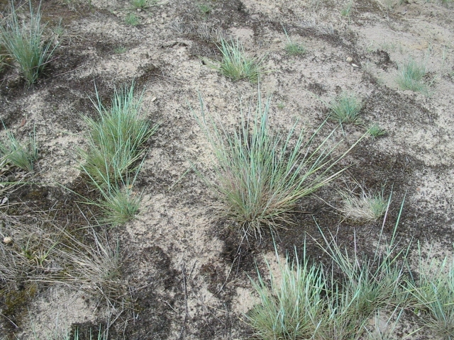
The application Bio7 was originally developed for the chair of experimental and systems biology (Bio7) to create and analyze spatially explizit simulation models on dry acidic grasslands on inland sand dunes. Only specialists like Corynephorus canescens, Polytrichum piliferum, etc. can settle on this nutrient poor water limited sandy soils. Additionally high temperatures on the surface of the soil and erosion make it very hard for other species to settle there. In comparison to other ecosystems this habitat is less complex in its species structure and nutrient dynamics which facilitates monitoring of vegetation dynamics to identify the driving forces or key factors of the system. With the exploration of this ecosystem several questions and hypothesis should be answered and verified. Because many specialized plants and animals occur in this habitat the main question is, how we can protect and preserve this valuable ecosystem at all. Also the key factors are from high interest and can maybe serve to identify similar processes in more complex systems like the tropical rainforest. From various experiments in these systems we have knowledge about seed dispersal, competition, and nutrients availability or dependencies from different species which are typical for this habitat. We use the capabilities of this application to express the features of this system in syntactical rules for simulation.
2 Getting started
2.1 Installation
2.1.1 System requirements:
It is recommended that your computer should have at least 1024 mb ram and a 1 ghz processor. A 3d Graphics Card which is OpenGL enabled (only necessary for the “Spatial” view and the embedded “WorldWind” view. To use the LibreOffice feature of Bio7 an installation of LibreOffice >= 4.0 is required. The path to LibreOffice will be automatically fetched by Bio7 from the registry (Windows) or can be adjusted in the Bio7 preferences (Windows, Linux, MacOSX) to the default path.
2.1.2 Installation:
2.1.2.1 Windows
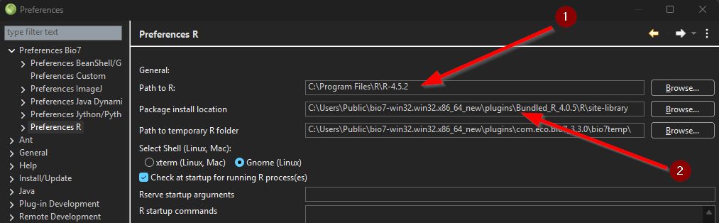
Just download the *.zip distribution file from the Bio7 Github Releases (https://github.com/Bio7/bio7/releases) and unzip it in your preferred location (avoid spaces in path!). Bio7 comes bundled with Java Adoptium and works out of the box. R and Rserve is not bundled (since Bio7 3.6) anymore by default! Download and install R and adjust the R path in the Bio7 preferences (optional also the default R packages path): Preferences->Preferences Bio7->Preferences R
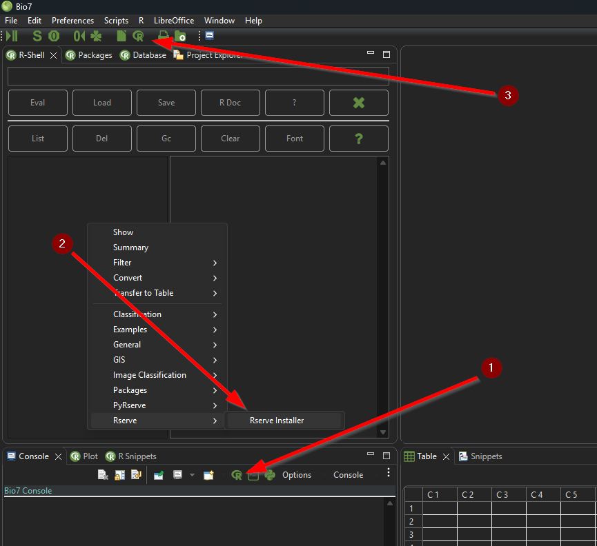
Install the Rserve package in R (no special Rserve version needed - see below Linux and MacOSX). For the Rserve installation you can also execute a Groovy script in the R-Shell-view after the R installation (start R in the Bio7 console).
2.1.2.2 Linux
Download and extract the installation file from Bio7 Github Releases. Bio7 comes bundled with Java (Adoptium). Please note that you have to start Bio7 with Xorg (X display server) because of SWT_AWT which is used by ImageJ. For Linux you have to install R and a special compiled version of Rserve. The default OS path to R is used automatically if not set (like in Windows) in the preferences. Simply execute an available Groovy script in the R-Shell view (see Windows notes above).
To install Rserve manually start the R console and paste the following command, see:
https://github.com/Bio7/Rserve-Cooperative
To install Rserve manually start the R console and paste the following command, see:
https://github.com/Bio7/Rserve-Cooperative
2.1.2.3 MacOSX
Download and extract the installation file from Bio7 Github Releases. Bio7 comes bundled with Java (Adoptium). For MacOSX you have to install R and a special compiled version of Rserve. The default OS path to R is used automatically if not set (like in Windows) in the preferences. Simply execute an available Groovy script in the R-Shell view (see Windows notes above). To install Rserve manually start the R console and paste the following command, see:
https://github.com/Bio7/Rserve-Cooperative
To start Bio7 (unsigned) on MacOSX:
To start Bio7 after installation please follow this advice (sign app locally):
https://github.com/Bio7/bio7/discussions/30
https://github.com/Bio7/Rserve-Cooperative
To start Bio7 (unsigned) on MacOSX:
To start Bio7 after installation please follow this advice (sign app locally):
https://github.com/Bio7/bio7/discussions/30
2.1.2.4 Rserve local installation (compiled for cooperative mode on Linux and MacOSX, 64-bit platforms)
Manual local installation on Windows, MacOSX and Linux from R command line (please adapt the file path!):
1install.packages("C:/xxx/Rserve_1.8-8.zip", repos=NULL)
Figure 2.3 R command to build Rserve (from an archive)
MacOSX:
1install.packages("/Users/xxx/Rserve_1.8-8.tgz", repos=NULL)
Figure 2.4 R command to build Rserve (from an archive)
Linux (Compiled with Ubuntu 20.10):
1install.packages("/home/xxx/Rserve_1.8-8.tar.gz", repos=NULL)
Figure 2.5 R command to build Rserve (from an archive)
2.1.2.5 Build of Rserve in cooperative mode on Linux or MacOSX (if necessary!)
1sudo PKG_CPPFLAGS=-DCOOPERATIVE R CMD INSTALL --build Rserve_1.8-8.tar.gz
Figure 2.6 R command to build Rserve (from an archive)
1sudo PKG_CPPFLAGS=-DCOOPERATIVE R CMD INSTALL --build Rserve
Figure 2.7 R command to build Rserve (unpacked)
2.1.3 R Windows specific:
The default add-on package location in a Bio7 release is now: “Bio7\plugins\Bundled_R_x.xx.xx\R\site-library”. At this location inside of Bio7 the packages will be installed by default (if not changed!).
2.1.4 Useful R packages
To use all Bio7 functions ( for editor formating, knitr documents, markdown documents, spatial analysis and import, export of spatial data) some R packages are recommended and required to install.You can install all packages e.g. with a R script available in the R-Shell view context menu of Bio7 (Packages->Install_Default_R_Packages)
2.1.4.1 R packages Linux specific:
For Linux there are no binaries available. For the compilation of the R packages the Linux packages g++ and gfortran have to be installed (if not available by default!). For the compilation of the rgdal package in addition you need the Linux packages: gdal, libgdal-dev, libproj-dev. If you would like to install the spatstat package, too, you need: libblas-dev,liblapack
2.1.5 R Markdown
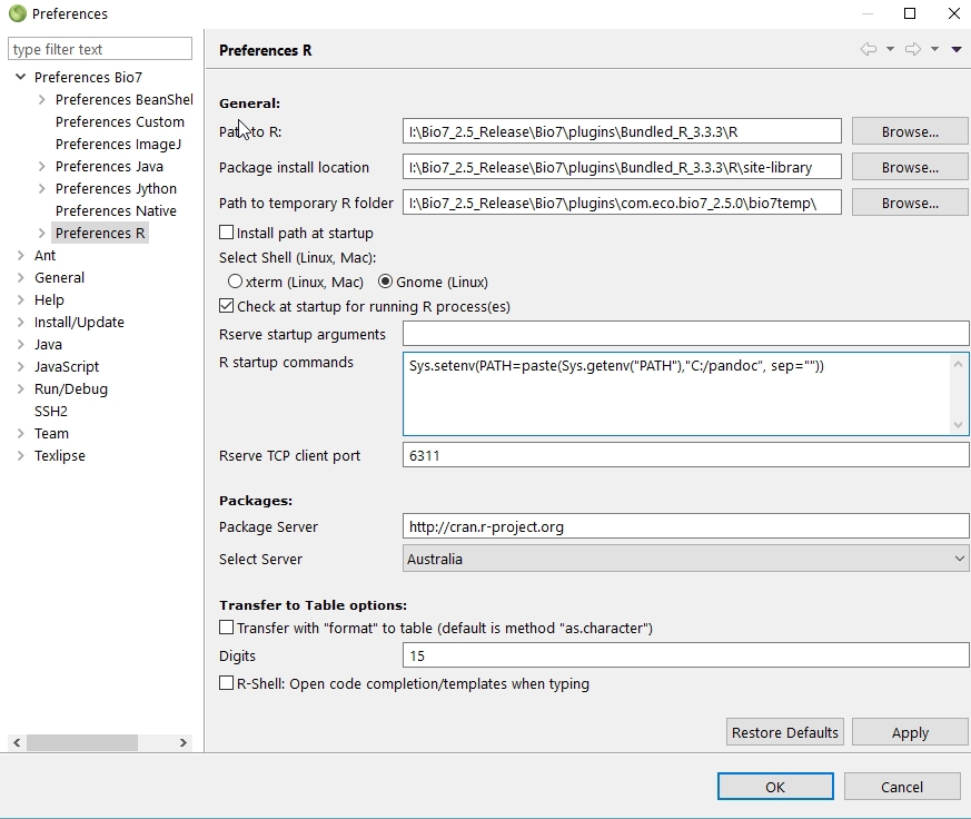
To use the R Markdown features please install the rmarkdown package, knitr from within R and the pandoc binaries from here: https://github.com/jgm/pandoc/releases/latest For Windows and MacOSX pandoc must be on the system PATH – Linux adds the path by default! You can also add the path in R with:
Add pandoc to the OS PATH. Else type in the R console:
1Sys.setenv(PATH="/usr/bin:/bin:/usr/sbin:/sbin:/usr/local/bin")
Figure 2.8 R command to set OS PATH in R only
1Sys.setenv(PATH="/usr/bin:/bin:/usr/sbin:/sbin:/usr/local/bin:$HOME/bin")
Figure 2.10 R command to set OS PATH in R only
Add pandoc path to the Windows PATH if necessary (evtl. restart). Else type in the R console:
1Sys.setenv(PATH=paste(Sys.getenv("PATH"),"C:/pandoc”, sep=""))
Figure 2.11 R command to set OS PATH in R only
2.1.6 LaTeX
To use LaTex with Bio7 please install a LaTeX environment e.g.:
MiKTeX (http://miktex.org/)
MacTeX (https://tug.org/mactex/)
TeX Live (http://www.tug.org/texlive/)
2.1.6.1 Linux
To compile markdown documents with pdflatex two packages seems to be required from texlive
2.1.7 Portable (Windows):
It is also possible to install Bio7 on an Usb-Stick with the described procedure. Moreover LibreOffice can also be installed portable with Bio7. Download the portable version (http://portableapps.com/apps/office/libreoffice_portable) and adjust the LibreOffice path to the LibreOfficePortable\App\libreoffice\program subfolder in the Preferences.
2.1.8 Examples for Bio7:
On the Bio7 SourceForge website you can download examples for the Bio7 application. In addition the examples (https://github.com/Bio7/bio7_examples) can be accessed on github. To install the Bio7 examples please import the examples from the Examples.zip file. File\SpecialChar menuseparatorImport\SpecialChar menuseparatorExisting Projects into Workspace. Select the archive file Examples.zip and the two projects. Press Finish to import them into Bio7 (they will be imported to the workspace location). Please take care to import the examples as a *.zip file to restore the relative resource path of the examples (on MacoSX the examples are often unzipped after download. Please adjust the settings to avoid the decompression of the archive file).
2.1.9 Increased Java memory Windows/Linux
For an increased Java heap space open the Bio7.ini file in the install directory of Bio7. In the file you can change the default memory settings e.g. the initial heap size -Xms and the maximum heap space -Xmx.
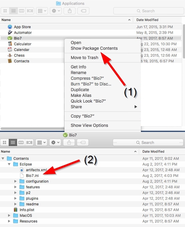
2.1.10 Increased Java memory MacOSX
For an increased Java heap space open the Bio7 package (context menu if you click on the icon) then go to Contents/MacOSX and open the Bio7.ini file with a text editor. In the file you can change the default memory settings e.g. the initial heap size -Xms and the maximum heap space -Xmx
3 The Platform-Architecture
After the Bio7 application has been launched a typical Eclipse workbench window is displayed. An Eclipse window contains a page, which contains an arrangement of views and editors whose layout is defined by a perspective.
3.1 The Toolbar
The toolbar offers several default actions which are described in the following section.It should be noted that editors or plugins can add items to the toolbar.

3.1.10.1 Toolbar from left to Right:
- Play/Pause: Starts or stops a simulation run. This action will start or pause a default calculation thread of the application. The calculation thread then repeatedly calls a special method (called run) in a compiled Java class if available (which extends a special class called “Model”). In the submenu the Control view can be opened to change the execution interval of the calculation thread.
- Setup: Invokes a Java setup method if available in the compiled class.
- Reset: Resets the discrete grid (if opened) in the application. This action will reset all states in the Quadgrid (Hexgrid) arrays to the value 0.
- Counter-Reset: Resets the counter to null. This action will reset the time to the value 0 and will also update the default charts. The values of a special list which automatically stores the count of enabled states in a simulation run will also be deleted.
- Random: Distributes selected states in the discrete field (if opened). There are two random functions available in the menu of this item to randomize the field. With a special action landscape patterns can be produced (see 4.9.3↓).
- LibreOffice: This action will open a connection to LibreOffice. If you select this action Bio7 tries to connect to LibreOffice with the LibreOffice API (Application Programming Interface). The path to LibreOffice will be fetched from the Preferences and can be adjusted there (Windows: If LibreOffice is installed, it will be automatically fetched from the Windows Registry if possible. Sometimes the Windows path to LibreOffice has to be adjusted, too. With this connection some actions are available (see 9.3↓)
- R: Will open a connection to R by means of a Server (Rserve). This action will connect Bio7 to the Rserve application which builds a connection to the statistical tool R (see 4.6↓). In the submenu of this action the started R process can be terminated or killed if necessary.
- Print: Prints the content of an opened editor. If an editor in Bio7 has been opened this method will print the content.
- Create new Projects and Files: With this toolbar menu Bio7 projects with default files can be created easily without to create the project and files individually (fast mode).
Note: When a file has been opened additional entries occur according to the opened editor.
3.2 The Menu
The menubar of the Bio7 application offers several menus for the work with the different components of the application.
- The File menu offers methods for the import and export of projects and files which can be extended with BeanShell, Groovy or Jython scripts.
- The Edit menu offers several methods for the work with the different editors in Bio7.
- The Preferences menu opens the preferences of the Bio7 application (see 6.1↓).
- The Scripts menu (with several submenus) is extendable for self-defined scripts (BeanShell, Groovy, Jython, R scripts and ImageJ macros) in different categories.
- The R menu offers methods for the interaction with R and to transfer data to the embedded R application (see 4.6.1↓).
- The LibreOffice menu offers actions for acquiring and setting values from and to LibreOffice. Three further methods can transfer data to R or BeanShell which facilitates data acquisition through the options of LibreOffice application (see 9.3↓).
- With the Window menu perspectives and views can be opened and the editor area can be activated in a Bio7 perspective. In addition custom perspectives can be stored with an action available in this menu.
- The menu Help offers help for the application and the possibility to make updates and installations of new components for Bio7 (see 7↓).
4 The Perspectives of Bio7
In the perspective bar several different perspectives can be activated via the perspective buttons. All the views or editors in the perspective can be closed, opened, detached or moved. The perspectives in Bio7 can be extended with several other views which can be opened in the Windows\SpecialChar menuseparatorViews menu or with the default action in the status bar at the bottom left of the program. Additionally self defined perspectives can be created or deleted. From the Eclipse Workbench User Guide (http://help.eclipse.org): “Perspectives provide combinations of views and editors that are suited to performing a particular set of tasks....”
- Click the Open Perspective button on the shortcut bar on the left side of the Workbench window. (This provides the same function as the Window \SpecialChar menuseparator Open Perspective menu on the menu bar.)
- To see a complete list of perspectives, select Other... from the drop-down menu.
- Select the perspective that you want to open. When the perspective opens, the title bar of the window changes to display the name of the perspective. In addition, an icon is added to the shortcut bar, allowing you to quickly switch back to that perspective from other perspectives in the same window.
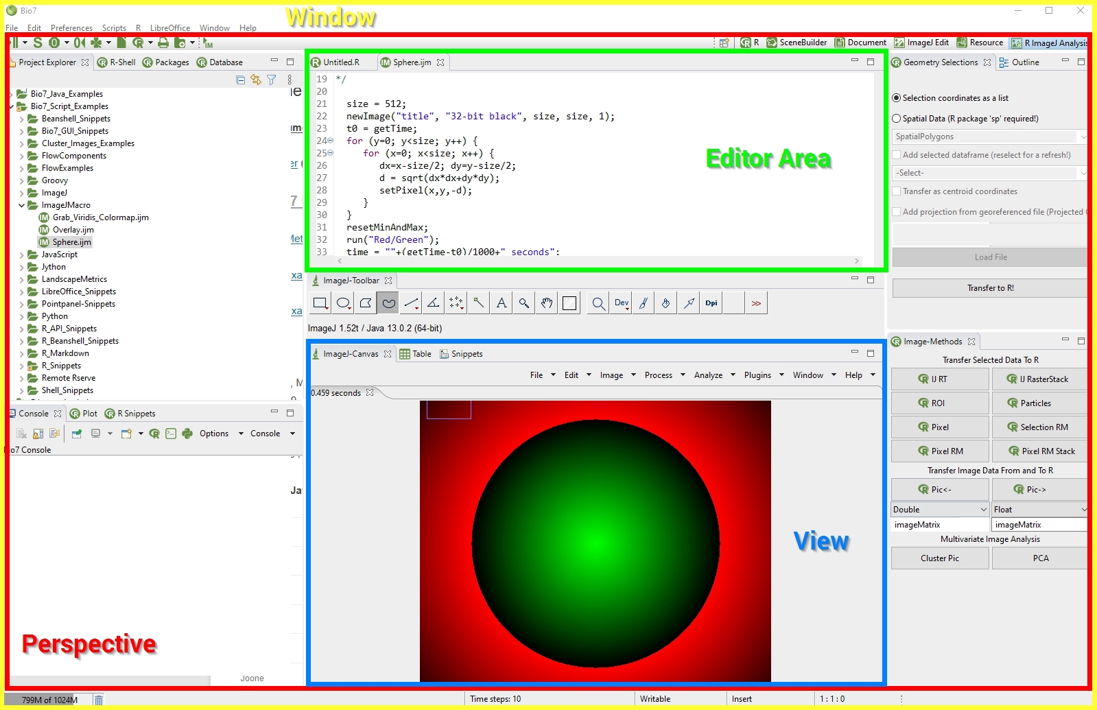
4.1 Resource Perspective
After Bio7 has been started the perspective in front is the Resource perspective. The parts of the Resource perspective are:
(1) The Navigator view to import, export, open and manage files.
(2) The Editor area where the editor files are opened.
(3) The Console of Bio7.
(4) The Outline view (active when an editor has been opened).
(5) The Properties view which shows the selected file properties (also important for the adjustment of the Flow editor properties).
(6) The Snippets view in which snippets for the different text based editors of Bio7 can be created.
(7) The context menu of the Navigator view which contains several file actions. Some actions are only visisble if a special file type is selected (e.g. the R Packages action in the screenshot is only visible when a R file is selected).
4.1.1 The Navigator
In the Navigator view files can be managed and stored. The context menu offers several actions to import and export files for the available Bio7 editors and specialized actions dependant on the selected filetype. All the files are managed by projects which can have folders and subfolders, etc. for managing a large amount of different files. These projects and their files can be exported or imported as *.zip files for data exchange. The file navigator (Navigator view) of Bio7 allows you to create different editor files with a help of a file wizard. A double-click on the file in the file navigator will open the file in the default registered editor.
4.1.2 The Editor Area
The editor area is the area where all files are opened and edited. The context menu varies depending on which file is opened. When opened the text based editors offer typical text functionalities like: Copy, Paste, Undo, Redo, Cut, Find/Replace, Print, etc. in the context menu and in the edit menu (menubar) of Bio7. When a file has been opened editor specific buttons will be added to the toolbar which execute an editor action according to the opened file (compilation respectively interpreting code of Java, BeanShell, Groovy, Jython , R or execution of a Flow!). The editor area can be enabled in every perspective with the Window\SpecialChar menuseparatorShow/Hide Editor action in the main Bio7 menu.
4.1.3 The Console of Bio7
The Bio7 console gives access to several interpreted languages and a pseudo-terminal for the Operating System (OS) environment. In the view menu the different modes can be selected.
- The script consoles (Beanshell, Groovy, Jython) can interactively communicate with the Bio7 application or simply interpret different instructions in the selected scripting language.
- The Shell pipes commands to the underlying OS with a pseudo-terminal.
- The Native R and Native Python consoles pipe commands to the different applications (Please adjust the paths to the language environments in the Preferences! See: 10.1↓).
-
The default enabled Console Output only displays errors and prints messages. In addition it pauses the REPL (read–eval–print loop).The Console is responsible for the:\begin_inset Separator latexpar\end_inset
- Output messages for the interpreters and connected applications.
- Output messages of the embedded Java compiler (compiler warnings, infos, etc.)
- Output of the R interpreter (Rserve warnings, etc.) and evaluated expressions in R.
In the context menu of the Console view several actions are available to clear displayed text or copy text from the console to the clipboard.
4.1.3.1 Menu of the Console View
In the Options menu of the Console view text encoding properties, font settings and special interpreter commands can be selected. As already noted in the Console menu the different interpreters and native connections (R, Python, OS shell) can be selected.
4.1.4 The Snippets View
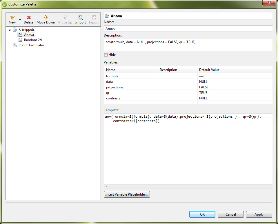
In the Snippets view code templates can be created and stored for the different editors in Bio7. The Snippet view plugin comes from the WTP project (https://eclipse.org/webtools/wst/components.html). To create snippets inside this view, categories have to be created inside a template editor (Customize... action in the context menu). This editor can be opened with a right-click in the Snippets view. Copied text from any text based editor of Bio7 can be pasted directly as a snippet after a category has been created inside the view. In addition selected text in an editor can be stored as a template. More complex templates with variables and a detailed description can be created, too. This is extremely useful if you want to create custom formulas or statistics. A created template can be transferred to an active opened editor with a double-click of the mouse device. Optional the different categories can also be folded and customized for a better overview (see figure below).
4.2 ImageJ Edit Perspective
The Image Edit perspective is the default perspective to perform Image Analysis and supports the creation of ImageJ macros, scripts or Java plugins. ImageJ macros, etc., can directly be opened and edited in a Bio7 supported ImageJ editor (BeanShell, Groovy, Jython, JavaScript, ImageJ Macro, Java plugins) opened from the Navigator view on the left and executed with the dedicated interpret action in the main Bio7 toolbar. The arrangement of views in this perspective was optimized for an typical image analysis workflow. The ImageJ view on the right side is described in 4.4.1.
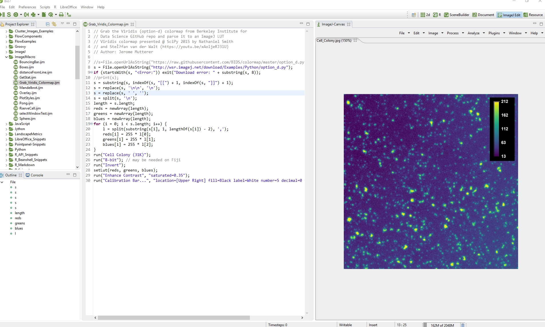
4.2.1 ImageJ-Canvas
For a complete description of the software ImageJ follow the link: http://rsb.info.nih.gov/ij/. The online documentation can be found here: http://imagej.nih.gov/ij/docs/guide/index.html. The differences between the regular version of ImageJ and the integrated version in Bio7 are described in the list below:
- The ImageJ canvas is embedded in Bio7 as a tabbed SWT interface.
- The Toolbar of ImageJ is integrated in an RCP view (when called from the menu Window\SpecialChar menuseparatorImageJ-Toolbar as a detached view).
- Two extra actions have been added to compile or interpret current opened sourcecode on the ImageJ classpath only (OSGI seperated plugins classpath: Plugins\SpecialChar menuseparatorCompile Java and Plugins\SpecialChar menuseparatorInterpret Script)
- Several actions for the image data transfer to R are available in a special detached view (see 4.8↓)
- The menu of the integrated application has been reprogrammed as a SWT view menu which is similar to the original ImageJ menu.
- All images are opened in tabs and can be edited if activated.
- External plugins are supported. Installed plugins extend the ImageJ menus of Bio7 ImageJ view dynamically.
- The menus can be updated dynamically (if a new plugin has been added) with the “Refresh Menus” action.
- Macros can extend the main menu of Bio7 and can be created like in the regular version.
- For more information about these plugins visit the different websites (for available manuals!).
- The ImageJ API is accessible by means of the embedded compiler or with BeanShell, Groovy, JavaScript, ImageJ Macro or Jython scripts.
As aforementioned functions of ImageJ can be called directly from the Java compiler or from the different interpreters. Many of the available examples from the ImageJ website can be executed directly within the different editors of Bio7 by compiling or interpreting them. All standard functions of ImageJ are integrated. Macros are fully supported and can also be added dynamically to the main menu of Bio7 for customized actions. In the menu of the ImageJ view some additional menu points (“Windows “) have been added for:
- Opening the toolbar of ImageJ (ImageJ-Toolbar as a detached view - see below)
- Opening a control panel for the Points panel with methods for the exchange and adjustment of images between ImageJ and the Points panel.
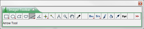
4.2.1.1 ImageJ Toolbar
As already noted the ImageJ toolbar is integrated in Bio7 as a view. It will be opened detached if the the ImageJ toolbar action is executed (Window\SpecialChar menuseparatorImageJ-Toolbar). Drag and drop actions (open images and install ImageJ plugins) are supported, too. In addition macros for the toolbar can be installed (as known from ImageJ).
4.2.1.2 ImageJ Plugins And Macro Paths
Bio7 supports plugins and macros for ImageJ. The default paths to the macros are:
- Bio7/plugins/com.eco.bio7.image_x.xx.xx/plugins
- Bio7/plugins/com.eco.bio7.image_x.xx.xx/macros
If plugins are dropped in the plugins directory the menu Plugins will be extended with submenu actions. In addition the Plugins\SpecialChar menuseparatorUtilities\SpecialChar menuseparatorControl Panel action is available to display all installed plugins. For more information about plugins and macros please consult the ImageJ documentation.
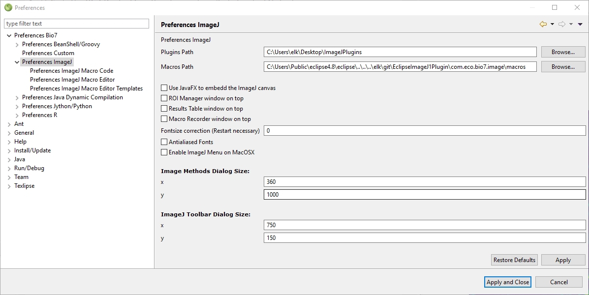
4.2.1.3 ImageJ preferences
In the ImageJ preferences several values can be adjusted. For instance the path to the plugins and macros can be changed as well as some preferences of the ImageJ macro editor (editor colors, code preferences,templates, etc.).
4.2.1.4 Compilation of ImageJ plugins
The compilation of ImageJ plugins can be done with the default ImageJ compile action in the Image-Canvas menu (e.g. Plugins\SpecialChar menuseparatorNew\SpecialChar menuseparator Plugin) or with the Java editor of Bio7. In the File creation wizard of Bio7 ImageJ plugin and filter templates are available.
4.3 R ImageJ Analysis Perspective
A special perspective is available to combine scientific image analysis with statistical analysis. In this perspective the R and ImageJ tools are arranged side by side for an easier access.
4.3.1 ImageJ Interactions with R
In Bio7 a special view is available (ImageJ-Canvas menu->Window->Bio7-Toolbar) which offers several actions to transfer Imagej image data to and from R. The availabe actions are described in the following list.
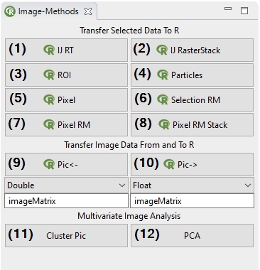
(1) This action transfers all values of an opened ImageJ Results Table to R as a dataframe object.
(2) The ’IJ Raster Stack’ action transfers an opened ImageJ stack as a list of matrices or ’RasterStack’ to R. The datatype can be selected, too (see datatype in 9).
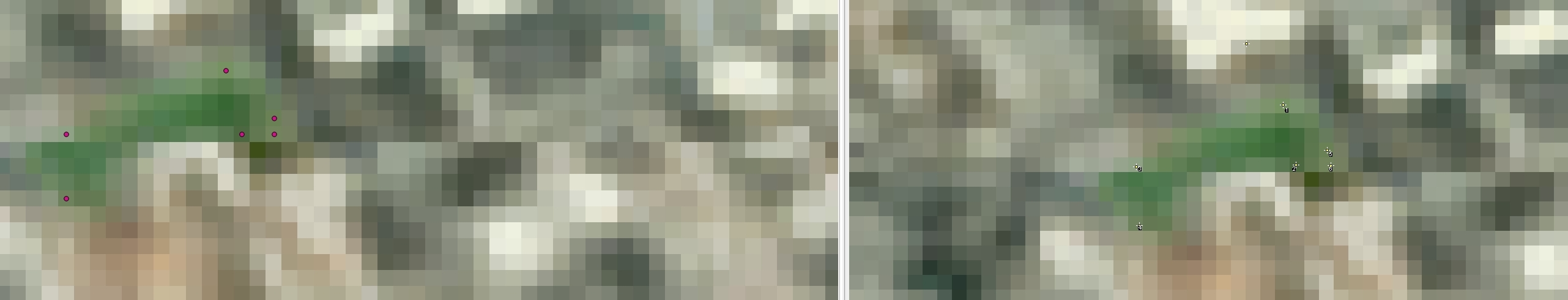
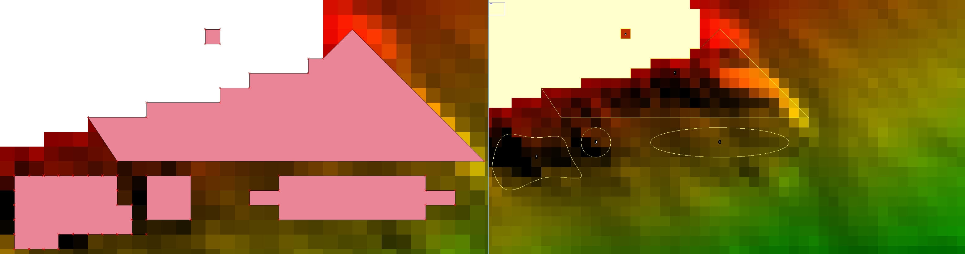
(3) This action transfers single ImageJ selections (ROI’s) x,y-coordinates to R.
(4) This action opens the “Particle Analysis” dialog of ImageJ. If the particle analysis is executed the results of the analysis are transferred to R as a dataframe.
(5) Transfers the selected pixels (Freehand, Rectangular etc.) with or without a signature as a matrix to R. The transfer type can be selected, too (see datatype in 9)!
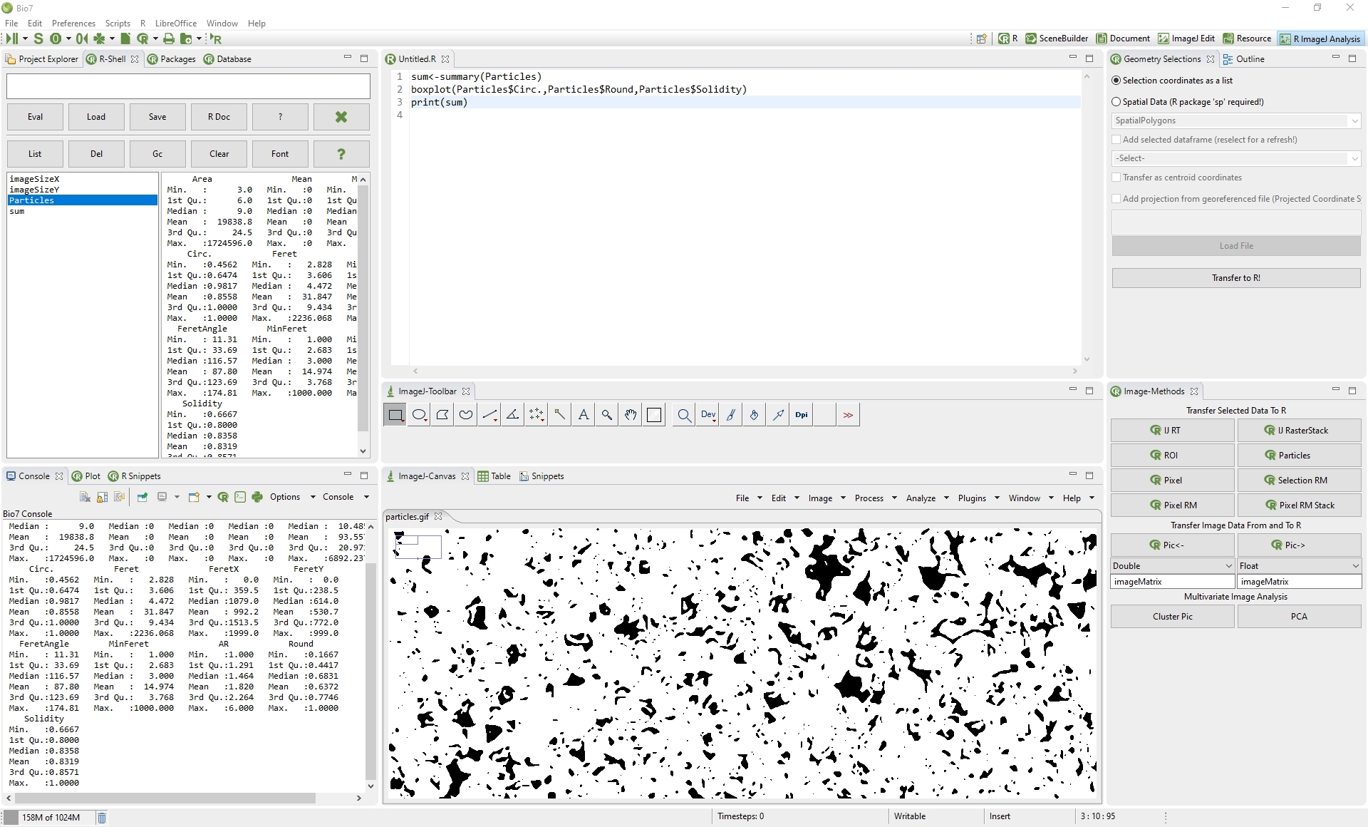
(6) Opens the Geometry Selections view (already visible in this perspective) which offers different actions to transfer selection data (coordinates) as R data (x,y or georeferenced!).
(7) Transfers multiple selected pixels (Freehand, Rectangular etc.) with or without a signature from the ROI Manager as a matrix to R. The transfer type can be selected, too!
(8) Transfers multiple selected pixels (Freehand, Rectangular etc.) of a stack with or without a signature from the ROI Manager as a matrix to R. The transfer type can be selected, too!
(9) This action transfers the current image data of various types of ImageJ to R. The transfer name can be given in the textfield and the datatype in the combobox below. A matrix transfer is optionally possible if the datatype double is selected.
(10) This action creates an image of a selected R matrix or vector (exisiting R object name must be given in textfield below). The datatype of the ImageJ image type (Color, Greyscale, Float, Short) to ImageJ must be choosen in the combobox below.
(11) Action to perform a cluster analysis. Creates a new image from the assigned pixels.
(12) Action to perform a PCA analysis. Creates a new image from the assigned pixels.
4.3.1.1 Image Transfer to R
With the actions (9) (10) the data of the current active image can be transferred to R or image data from R to ImageJ in a selected datatype, respectively image type. It is good practice to transfer the image data in the less consumptive data type needed for a transfer. In addition special transfers are available for selected image data:
- The action in (5) transfers selected image data in an easy way without the need of an opened ROI Manager in ImageJ. The image data of the current selection (one selection) from one or multiple images (opened tabs) can be transferred to R in the selected datatype of the combobox of action (9).
- The action in (7) transfers the selected pixels (Freehand, Rectangular etc.) with or without a signature as a matrix to R. The transfer type can be selected, too! The ROI Manager with ROI selections has to be active. Selected ROI Manager ROI selections (or all ROI’s if no ROI is selected) for all layers (opened tabs in the ImageJ view) are transferred automatically with an selected or incremental signature! If a stack is among the opened images only the first slice (layer) will be transferred.
- The action (8) transfers the selected pixels of the selected ImageJ selections (Freehand, Rectangular etc.) in a stack with or without a signature as a matrix to R. The transfer type can be selected, too! The ROI Manager with selections has to be active and the selected image must be a stack! All selections for all slices are transferred automatically with an selected or incremental signature! A stack can also represent multispectral or hyperspectral image data which selectively should be transferred to R! Note that image folders can be dragged on the toolbar or the ImageJ canvas to load the images as a regular or virtual stack (in a virtual stack only the displayed data is loaded into the RAM of the computer).
Note: A description of the ROI Manager for action (6), (7) and (8) can be found here: http://rsbweb.nih.gov/ij/docs/guide/146-30.html#sub:ROI-Manager...
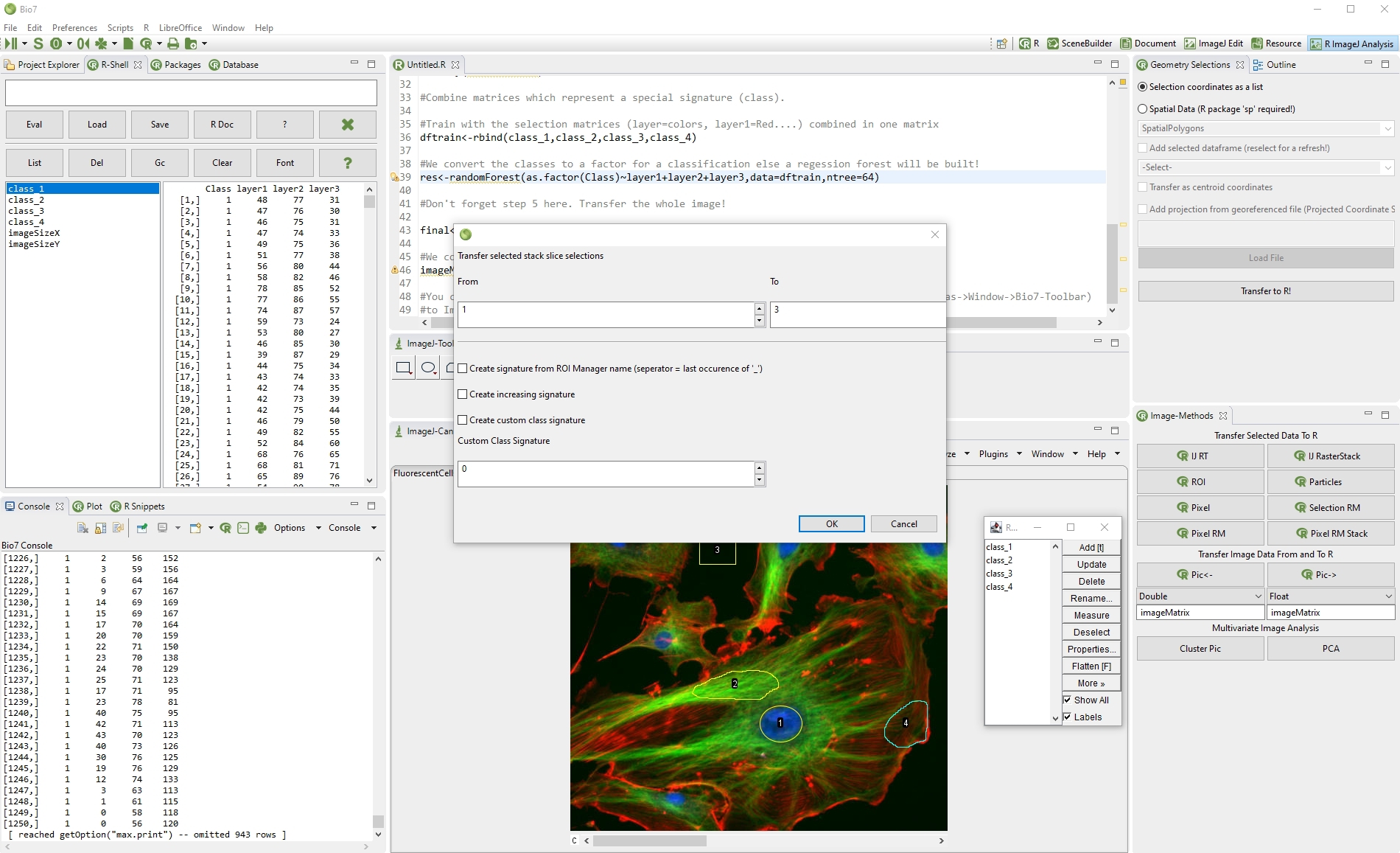
4.3.1.2 Supervised Classification with ImageJ and R
The options to create custom class signatures in action (7) and (8) is especially useful if a supervised classification of image data in R should be performed. Every ImageJ selection could represent a special vegetation or tissue type (e.g. class plant species, class tumor) represented by multiple spectral bands respectively available data (slices in the stack) which could be used for a training phase of supervised classification. See Bio7 programming examples: https://github.com/Bio7/Bio7.
4.3.1.3 Transfer of Selection Coordinates
As already noted with the actions (3) single and (6) multiple selection coordinates can be transferred to the R workspace. This is useful if you want to perfom e.g. shape analysis or morphometrics.The selection coordinates are transferred in integer precision. ImageJ also has some nice actions available to edit the selections. They can be found in ImageJ-Canvas menu under Edit\SpecialChar menuseparatorSelection. For example imprecise selections can be interpolated with a spline action or a Convex Hull can be created from a selection to reduce the amount of data points.
4.3.1.4 Geometry Selections View
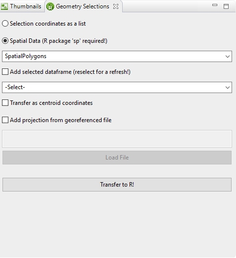
As already noted the Geometry Selections view can be opened with the Selection RM action (6) of the Image-Methods view. The view offers several actions to transfer selection data:
- Selection coordinates as list: If this option is selected selections from an available ROI Manager of ImageJ are transferred as a simple 2D list to R.
-
Spatial Data (R package ’sp’ required): If this option is selected data can be transferred with the ’sp’ R package as the following objects in R:\begin_inset Separator latexpar\end_inset
- SpatialPolygons or SpatialPolygonsDataFrame (if an available R dataframe has been selected - Add selected data frame action!)
- SpatialLines or SpatialLinesDataFrame (if an available R dataframe has been selected- Add selected data frame action!)
- SpatialPoints or SpatialPointsDataFrame (if an available R dataframe has been selected- Add selected data frame action!)
The option Transfer as centroid coordinates transfers the selections as centroids of a grid cell instead of the top-left coordinate of a grid cell. This can be useful or necessary for point data to transfer the point selections in the center of a grid cell (see 4.11↓)! The option Add projection from georeferenced file allows the georeferenced transfer of the selection data from an raster image (e.g., *.geotiff). Please note that the file has to be in a projected into a Projection Coordinate System! Typically the image selection data originates from a georeferenced image which then is selected with the Transfer to R! action to extract the spatial information for the creation of a georeferenced spatial object in the R workspace.
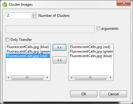
4.3.1.5 Cluster And PCA Analysis
As noted above the action to transfer selected image data can be used to perform a supervised classification with the availabe options. The actions described in (11) and (12) open special dialogs to perfom unsupervised classification (algorithm clara and kmeans) and a Principal Component Analysis (PCA) of the image data. In the dialog the number of clusters (PCA components) can be specified and arguments can be added to the default settings. Selected layers (opened images) can be added for the analysis. The Only Transfer option can be used to transfer the image data to R without performing an analysis. Please note that the selected image type (9) wisely choosen for a task can drastically reduce the amount of memory used for the analysis.
4.3.2 Thumbnails
With the thumbnail browser it is possible to open a directory of images as thumbnails. Open the context menu of the Navigator view and execute the menu action ’Open in Thumbnail view’ on a selected directory to preview images or LUT’s (Look Up Tables) in a split panel view. Different options are available for the display of thumbs.
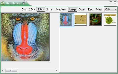
- With the 5->,10->, 15-> buttons you can select how many thumbs should be created in a row
- The Small, Medium, Large labelled buttons will create preview images with a size of 100*100, 150*150 or 200*200 pixel.
- The Open button opens the directory which should be displayed.
- The Mag. button enables or disables the overview navigation panel.
- The Rec. button enables the recursive search for images in selected folders (up to 1000 images!)
- The combobox will adjust the level of magnification. The thumbs will be resized by means of the lens (blue rectangle in the right panel for the overview!).
Images or file extensions in the following formats will be opened (default ImageJ types):
- *.gif, *.jpeg,*.png, *. bmp,*.tiff (with preview!)
- *.pnm, *.pcm (without preview!)
- *.txt (e.g. macros, results!)
- *.roi (single ROI!)
- *.zip (Stacks, ROI Manager files!)
- *. LUT (Pseudocolor Image Look-Up Tables - A pseudocolor image is an image (8, 16 or 32-bit) with a look up table color assigned to it.
When you open a LUT directory pseudocolor images are created as thumbnails from a template image to visualize the applied LUT. The LUT can be assigned to an opened 8, 16 or 32-bit single channel image in ImageJ when pressing the thumbnail preview image in the left panel. Hoovering over an image will display the image information in a popup panel.
4.3.2.1 Mouse Actions Thumbnails Browser
The images can be opened in the ImageJ view by selecting the thumb image buttons in the left panel (left-click!). If you set the mouse over a thumbnail some information about the image will be displayed. A right-click of the mouse over an image opens the parent folder of the image.
4.4 The 3d Perspective
With Bio7 custom 3d visualisations are possible in a specialized OpenGL panel which eases the development of 3d models. In addition custom methods are available to easily load 3d models ,textures, custom shapes as well as libraries for geometrical measurements. The drawback of this flexibility is that the user has to take care of certain circumstances which accompanies the direct use of OpenGL (e.g. if using the Fullscreen feature which retriggers the internal init method).The 3d perspective can be enabled in the perspective bar of Bio7.
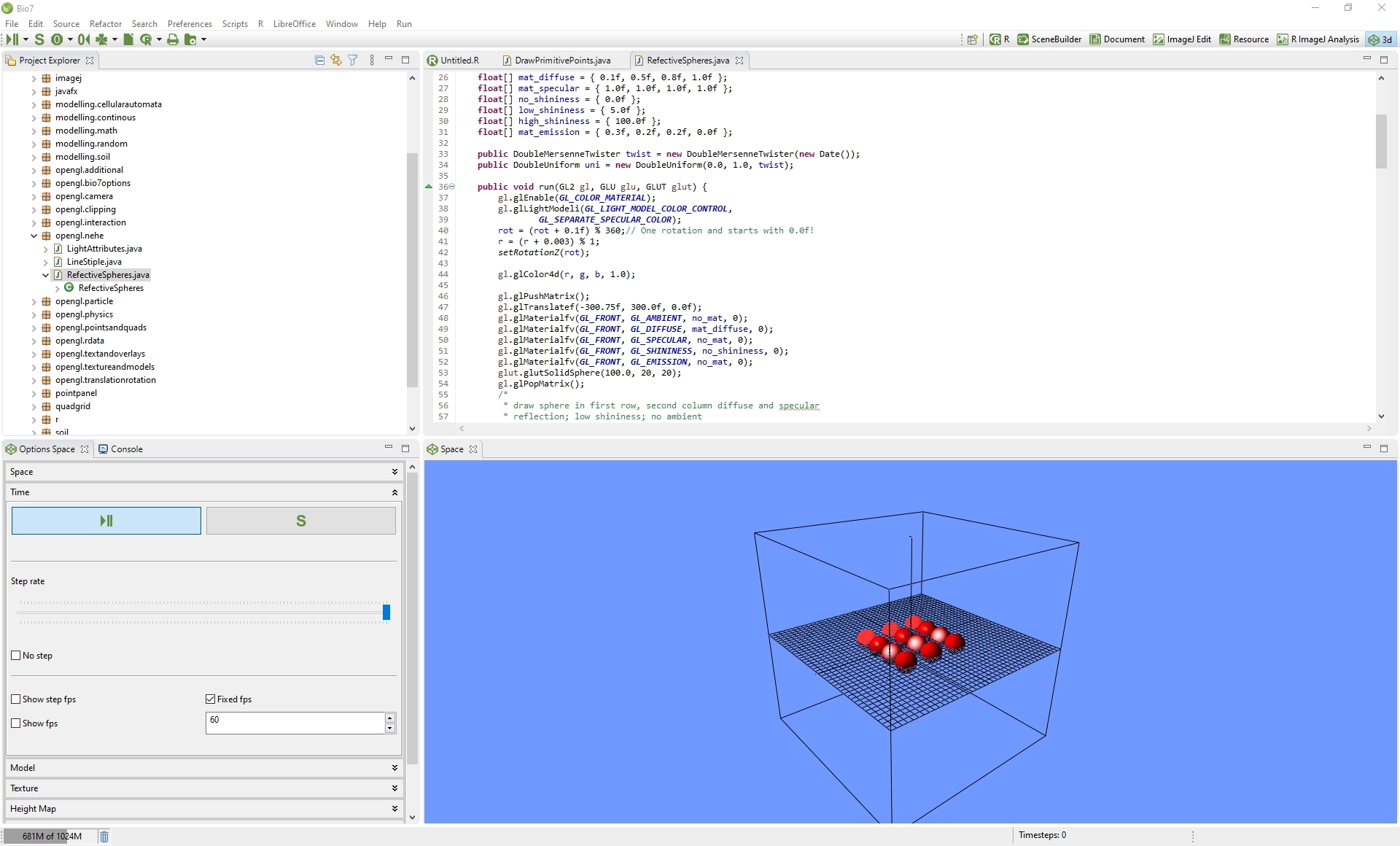
4.4.1 The Space View
The Space view is a new view in Bio7 which is enabled by default when the 3d perspective is opened. Aspects of this view can be controlled with the associated Options Space view which in addition is displayed by default in the 3d perspective. The Space view itself is an embedded GLPanel which visualizes OpenGL (Jogl) commands. After activation of the Space view a quad, the x,y,z coordinates of the world and a grid are shown for orientation. (the z-axis is pointing to the user - the OpenGL coordinate system is right-handed!). With the mouse device the visible world can be rotated (“Arcball” interface) easily - moved left, right and moved forward or backwards (see table below).
| Device | Event | Function |
| Left Mouse Button | Drag left, right,up,down | Rotation |
| Right Mouse Button | Drag left, right | Move forward, backwards |
| Middle Mouse Button | Drag left,right up, down | Move up,down, left, right |
| Key | F2 | Fullscreen |
| Key | Escape | Exit Fullscreen |
| Table : Interface Walkthrough (see Camera panel) | ||
| Left Mouse | Drag left, right, up, down | Rotation left, right, up, down |
| Key | PgUp, PgDn | Move up, down |
| Key | Arrow left,right | Rotation left, right |
| Key | Arrow up, down | Move forward, backwards |
Table 4.1 Interface Spatial view and Walkthrough interface
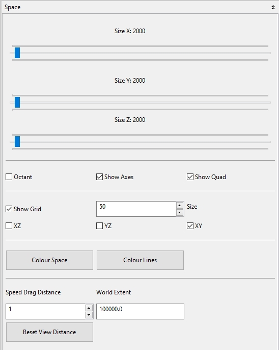
In the Options Space view several thematic panels can be expanded which offer different actions decribed below.
4.4.1.1 Time
After the compilation the execution must be enabled in the Time panel (Play/Pause). Also the Setup method (which invokes the method setup() in a compiled Java class if available) can be triggered here. The execution is separated from the normal execution of Bio7 to guarantee that the different thread are not mixed together which could result in an application crash. Furthermore the use of the animation timer guarantees a smooth animation of the developed model. It is very important not to trigger OpenGL methods from the regular execution thread of Bio7 that’s why these custom methods are available to access the full power of OpenGL (Jogl). If enabled the run method is triggered by means of the OpenGL timer and the default frame rate (as fast a the Graphics card allow it). The speed of the execution of the run method or the change of certain variables can be controlled by means of a custom method canStep() which switches a boolean value in dependence of a slider which is also available in the Time panel. Both frame rates, the regular execution speed (fps) and the speed of the triggered step (step fps) method can be visualized in the Space view. In addition a pause can be enabled (No Step) which switches the boolean of the canStep() method to false. If you want to control the speed of a simulation you can use the canStep() method to change values of variables (e.g. spatial coordinates) and hold them with the pause.

4.4.1.2 Space
In the Space panel of the Options Space view several adjustments can be made for the default components of the Space view. With the Octant action the default displayed grid is only drawn in the first octant (e.g. nice for a 3D plot). In additon some actions are available to select the colour of the space and to adjust the displayed grid (visibility, colour, size, etc.). The Fullscreen settings allow to adjust the screen resolution etc. before switching to the full screen mode (if available!). The World Extent sets the boundary space of the 3d panel (Universe) in which 3d objects coordinates will be displayed. With the Speed Drag Distance the speed for the default camera in z-direction can be adjusted. Reset View Distance resets the camera position.
4.4.1.3 Model
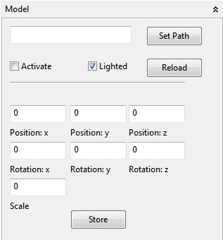
In the Model panel a default *.obj model can be loaded for a custom environment in a simulation or a visualisation of an 3d model. An *.obj model can be created e.g. with the 3D software Blender (also textured). By default several actions are available to scale and position the model in the Space view. These settings can be stored with the Store action (only integers will be stored!).
4.4.1.4 Texture
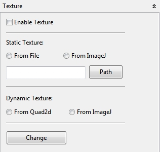
In the Texture view a default textured plane can be seleted (active ImageJ image or an imported image). In addition the Quadgrid or ImageJ image can be added as a dynamic (constantly redrawn) plane to the Space view. By default the texture plane is as big as the size of the image. The Change button is responsible to change the display to the selected texture source.
4.4.1.5 Height Map
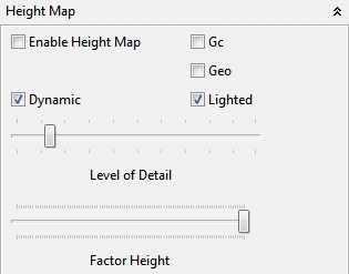
The Height Map panel can visualize a simple height map with height values of an enabled grayscale (8-bit, 16-bit, 32-bit) ImageJ image. The pixel values of the image determine the height of the height map. Some additional parameter control the resolution of the height map and a multiplying factor for the height. By default the height map is textured with the default selected image in the Texture panel (static or dynamic). Since the height map depends on an ImageJ image the image can be edited with ImageJ methods. Additionally an *.hgt importer script is shipped with Bio7 which creates a 32-bit image as a height map with correct height values in ImageJ.
4.4.1.6 Camera
With the Camera panel several aspects of the Space view perspective can be controlled. A Enable Walkthrough option enables a classical walk through perspective. If enabled you can walk through the Space view in the x,z plane. The walk directions (rotations up and down) can be controlled with the mouse and the arrow keys (see 4.4.1↑). The camera in this mode will always stay above the plane. This is not the case if the Enable Flythrough option is selected, too. Then the up and down movements of the camera changes the height position and the camera can also be moved below the plane - or negative height values. If the Custom camera is selected the camera can be positioned programmatically and it only shows the camera view if it is defined programmatically (and compiled!). With the Split View option an second camera can be enabled in the lower left of the Space view. In the text fields the position of the camera and the LookAt (the position to which the camera points) coordinates of the camera can be set (e.g. in double precision) and stored with the Store action. The last option Stereo enables an experimental Stereo renderer of the Space view for an anaglyph view of the Space.

4.4.1.7 Light
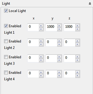
The Light panel controls the light of the Spatial view. Four different light source can be enabled and positioned with spinner fields. Please consider that the lights have a visible effect if more than one normal is defined for the surface (e.g height map, 3d models). If the Local light option is enabled (recommended!) the enabled lights will be rotated with the view.
4.4.1.8 Image
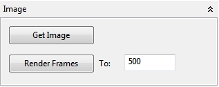
In the Image panel a screenshot from the current Space view can be transferred as an image to ImageJ. Furthermore it is possible to render a selectable amount of frames to ImageJ as an image stack which then can be saved as an *.avi file or an animated *.gif file. The size of the visible Space view determines the size of the images and the stack. A resize of the Space view automatically stops an active rendering to a stack.
If Fullscreen mode is supported the Fullscreen mode can be enabled with the F2 key, F3 key (secondary monitor) and quitted with the Escape key. This use of the fullscreen mode will trigger the setup method so it is important that certain objects are recreated in the setup method for the correct GL context (avoids a crash of the whole application!!! . TextRenderer objects, Texture objects and *.obj models should be created in the setup method with the correct gl context. Several example are available and demonstrate the general use of OpenGL inside of Bio7. Since OpenGL is single-threaded the Bio7 run method is executed from the internal OpenGL display method. The Bio7 Setup method is triggered from the internal OpenGL init method.
For a pain free use of OpenGL inside of Bio7:
- Please do not call an OpenGL method from a different thread.
- Generally create the following objects and models in the setup method: TextRenderer objects, Texture objects and *.obj models This ensures that the created objects in Fullscreen mode will be recreated with the correct gl context.
For more information about this read the Jogl User’s guide at: http://jogamp.org/ About Jogl in general the book of Andrew Davison: Pro Java 6 3D Game Development ISBN: 1590598172 http://www.apress.com/book/bookDisplay.html?bID=10256 Web Site for the book: http://fivedots.coe.psu.ac.th/~ad/jg2 (The *.obj loader source and part of walkthrough ideas are from this book which is highly recommended for an introduction of Jogl).
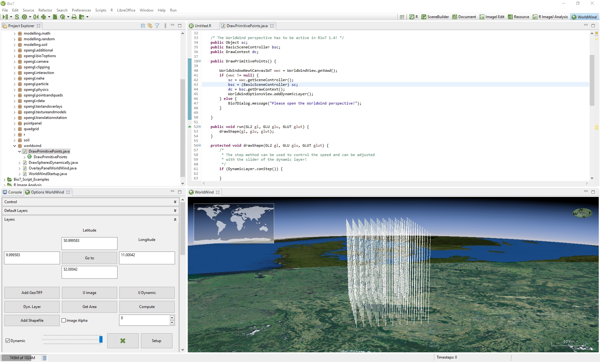
4.5 The WorldWind Perspective
The WorldWind perspective can be opened in the perspective bar. This perspective embedds two views, the Options WorldWind view (left) and the WorldWind view which embedds the NASA Java Virtual Globe “WorldWind” from: http://worldwind.arc.nasa.gov/java/. The Options WorldWind view offers several thematic panels and actions available if expanded.
Default Controls (description from: http://worldwind.arc.nasa.gov/java/)
| Pan | Left mouse button; click & drag - all directions |
| Zoom | Use the scroll wheel on the mouse or left & right mouse (both buttons); click & drag - up and down |
| Tilt | Right mouse button; click & drag - up and downor use "Page Up" and "Page Down" on the keyboard. |
| Rotate |
Right mouse button; click & drag - left and right
Note: Crossing the top and bottom half of the screen while rotating will change direction. |
| Stop | Spacebar |
| Reset Heading | N |
| Reset all | R |
| Fullscreen | F2, F3 (secondary monitor) |
| Exit Fullscreen | Escape |
| Visit List Locations | F4 |
Table 4.3 The Mouse with scroll wheel
| Pan |
Left mouse button; click & drag - all directions left mouse button
click once to center view. |
| Zoom | Hold "Ctrl" on the keyboard and left mouse button; click & drag - up and down |
| Tilt |
Hold "Shift" on the keyboard and left mouse button; click & drag - up and down or use
"Page Up" and "Page Down" on the keyboard. |
| Rotate | Hold "Shift" on the keyboard and left mouse button; click & drag - left and right |
| Stop | Spacebar |
| Reset Heading | N |
| Reset All | R |
| Fullscreen | F2 |
| Exit Fullscreen | Escape |
| Visit List Locations | F3 |
Table 4.4 Single mouse button
4.5.1 Control
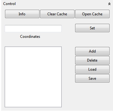
In the Control view custom coordinates or city names can be set in the Coordinates text field to navigate to the virtual location of the globe. The visible view (coordinates) can be stored for a later visit with a optional name. With the Clear Cache action downloaded textures (maps) can be deleted. The Open Cache action open the storage location of the textures. Coordinates of places can be stored between application sessions in the location list below the Coordinates textfield (Add). Selected list locations can be deleted with the Delete action. List coordinates can be exported or reimported with the Load and Save action. The coordinates are stored as a *.txt file. With the F3 key the list coordinates can be visited in order of the displayed list. This is very useful if you want to make a presentation in Fullscreen (F2) and visit several locations on the virtual globe. Note that you can also add image layers to the globe to enrich such a presentation with plots or visualizations.
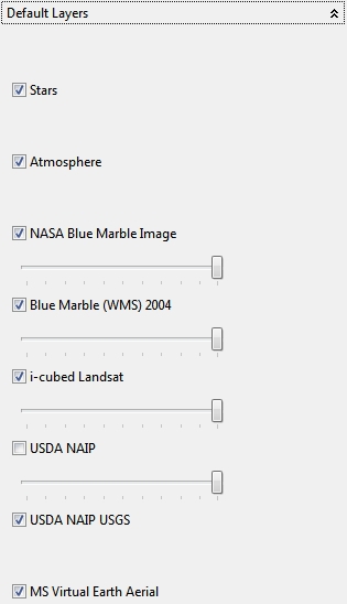
4.5.2 Default Layers
In this view special default available layers and maps from different sources can be enabled or disabled and blended together with an alpha value.
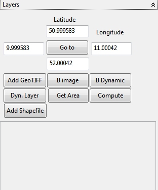
4.5.3 Layers
With this panel Shapefiles (Add Shapefile), GeoTIFF images (Add GeoTIFF), static (IJ image) or dynamic ImageJ images (IJ Dynamic - e.g. a animated stack) can be enabled on the WorldWind surface. In addition custom OpenGL visualizations can be compiled with the embedded Java editor and enabled as a layer (Dyn. Layer) on the 3D-globe. With the Latitude and Longitude textfields images can be referenced (positioned) on the globe and visited with the Go to action. The Get Area action fills the Latitude, Longitude textfields with information from special defined variables in R if available. So you can georeference images etc. in R, transfer the coordinates with the Get Area to the Latitude, Longitude textfields and then activate and position a selected layer on the coordinates (e.g. ImageJ images, R plots - ImageJ is the default R plot device!). With the Compute action coordinates (upper left and lower right) can be picked to set the Latitude and Longitude values in the textfields if the toogle is enabled (don’t forget to disable the toggle after selection!).
4.5.4 Render
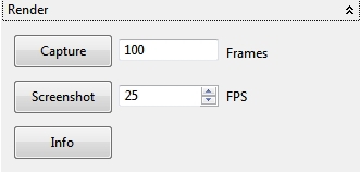
With the action Capture an animation of the globe can rendered to ImageJ. The amount of rendering time (Frames) and the framerate (FPS - Frames Per Second) can be adjusted, too. With the Screenshot action a screenshot of the panel can be sent to ImageJ as an image. The Info action shows some context help for the two actions.
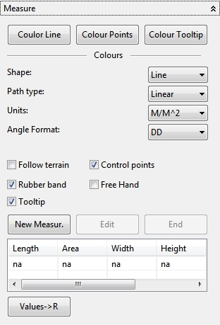
4.5.5 Measure
In the Measure panel some measurements on the globe can be made with different selection types. The Follow terrain options includes the height profile in the measurements. To start a new Measurement the New Measur. action has to be invoked. The selection type (Shape), path type (Path type), units (Units) and angle format (Angle Format) can be selected in available combo boxes before a measurement. Different measurements can be coloured with the actions Coulor Line, Colour Points and Colour Tooltip. With an available “Values->R” action the measurements can be transferred directly into a R workspace.
4.5.6 Projection
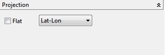
In the projection panel several globe projections can be selected with an option for a flat display (option Flat) of the globe.
4.6 The R Perspective and Menus
Bio7 embeds R as a statistical application to do profound statistical analysis of ecological models. To interact with the Bio7 application and all of its components the Rserve connection has to be started. In a start process the Bio7 application tries to connect to the Server (displayed in the progress dialog). If the connection trials exceed 10 trials (1/second) the operation will be aborted. After the connection has been established several methods for the interaction with R are available. By using the R editor (see 4.6.2.6↓) RScripts can easily be interpreted. Additionally some specialized methods are available in the R menu of Bio7.
4.6.1 R Menus in the Bio7 Main Menu
- Start Rserve starts R with a Rserve connection.
- With the Load Workspace action R workspaces can be loaded.
- The Save Workspace action saves the current workspace.
- Evaluate Expression opens a dialog where R expression can be evaluated. The evaluated expression will be displayed in the Console of the Bio7 platform.
- Evaluate Selection evaluates the selected line in the R editor and then jumps to the next line. In Rserve mode the line will be parsed and only evaluated if an expression is valid. Else it will be added to a string buffer until a valid R expression is given by the evaluated lines (use STRG+C or the R-Shell view action to interrupt!)
- The Evaluate Clipboard action evaluates R scripts which were transferred before to the clipboard.
- The Get Clipboard Data action will transfer data from the clipboard to the workspace of R and is stored in a dataframe “clip”.
- The action Remove all objects removes all objects from the current workspace.
- Start RGui with Workspace action starts the standard R shell or RGui with the current workspace if started on theWindows OS (The path to the temporary file can be adjusted in the Preferences of Rserve).
- The Preferences action opens the main R and Rserve preferences of Bio7
4.6.2 The R Perspective
The R perspective contains two views for the manipulation and analysis of data with R. The Table view for the import, export and transfer of data to R and the R-Shell view which embedds several methods and templates to evaluate and edit R data expressions.
4.6.2.1 The Table View
The Table view is a spreadsheet component in which data can be imported, exported, edited and transferred to R. Several sheets can be opened side by side as known from popular spreadsheet applications.
-
In the File menu the following imports and exports are supported:\begin_inset Separator latexpar\end_inset
- Import: Excel (1997-2007, 2010), CSV, Bio7 XML (to load formatted spreadsheets with images)
- Export Excel (1997-2007, 2010), Text, Bio7 XML (to save formatted spreadsheets with images)
- The Edit menu consists of several actions for copy and paste data, and edit sheet cells properties (color and size).
- The Sheet menu embeds several actions to create a new sheet, rename the sheet (or simply double-click on the tab!) or change the amount of rows and columns in the sheet.
- With the R menu data in the spreadsheet can be transferred to the R workspace as dataframes (with or without head) or as vectors of different types from selected data. Key combinations in a sheet work to select single values or portions of data (Strg + Mouse Click - select single cells, Shift + Mouse Click - select blocks). All cells of a row or column can be selected in the header (border) of the sheets.
- The Scripts menu can be extended with custom Groovy, BeanShell, Jython, R scripts (see ↓).
- In addition a context menu is available which support typical actions like cut, copy, paste and delete (the typical keys for those actions work, too - Strg+x, Strg+c, Strg+v).
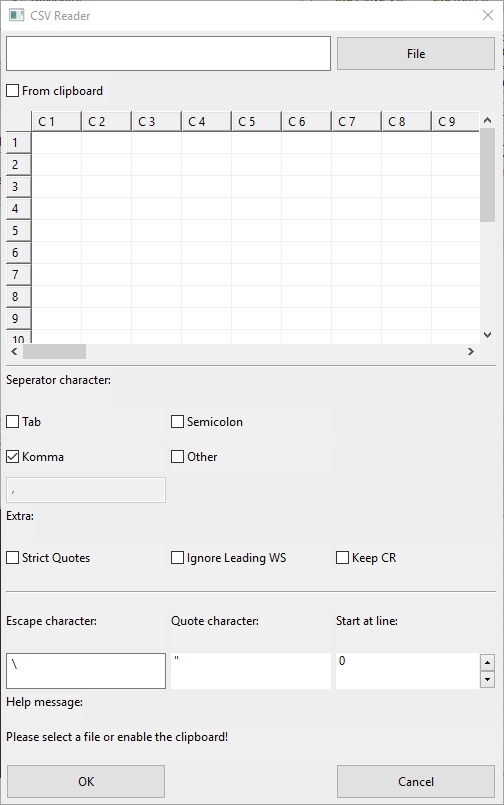
4.6.2.2 File Import for CSV Data
In the Table view menu a special import action is availabe to import *.csv files. Some configuration options in the dialog which will be opened with this action help in the configuration of a *.csv data import. With a preview action the consequence of e.g. changing delimiters and seperators can be visualized in a table.
4.6.2.3 The R-Shell View
The R-Shell view embeds an expression textfield and several tabs to manipulate, edit, transfer, plot data and templates for the R language.
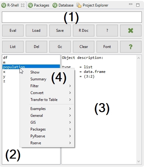
In the expression textfield (1) R expressions can be parsed and evaluated with the Evaluate Expression action. Parse errors are indicated in the top-left. Code completion is available by default with the key combination CTRL+SPACE. The history of the typed expressions are recorded and can be viewed with the arror-key (click to transfer the command to the expression textfield. Furthermore two actions are available to open the R documentation files. The actions below the textfield are listed here:
- With the Eval action valid R expressions (single and multiple seperated with a semicolon) can be evaluated.
- The Load and Save actions can save or restore evaluated commands stored in the available history (up to 100 commands!) of an R session.
- The RDocu action opens the documentation of R in an external Webbrowser.
- The ? action opens the documentation for a given keyword (package, method, etc.) in an internal webbrowser of Bio7.
In the data view (2) a context menu is available (see description below) to edit selected data types and transfer selected data to the Table view of Bio7. If a variable in the data view is selected an object description is given in the display of the right console panel. In the toolbar of the R-Shell view the following actions are available.
- The List action updates the data view of an active R workspace.
- The Del action removes selected data view variables (2) from the R workspace (single and multiple selections are possible! - Strg+left-click or Shift+left-click).
- The GC action triggers the garbage collection of R to free up space from the RAM.
- The Clear action clears the display (3) of the right console.
- The Font action opens a font dialog for the adjustment of the fonts in the data view and display.
- The ? action opens information about the use of the different actions available.
- Show - Displays the values of the selected variable.
- Summary - Summarizes the values of the selected variable.
- Filter - Filter actions for the R workspace to display only selected data structures.
- Converts - Actions to convert a variable to a selected datatype.
-
Transfer to Table - Actions to transfer data of the R workspace to the Table view of Bio7.\begin_inset Separator latexpar\end_inset
- Dataframe with Head: This action transfers a selected R workspace dataframe in the data view to the Table view in a new sheet. The first row will be transferred as the header.
- Dataframe: The same action as above but without a header.
- Matrix: This action transfers a selected R workspace matrix in the data view as a new sheet in the table view.
- Vector to Rows: This action transfers selected R workspace vector data to a row of a selected Table sheet starting at the selected table cell position of the sheet.
- Vector to Columns: This action transfers selected R workspace vector data to a column of a selected Table sheet starting at the selected table cell position of the sheet.
- Script Menus (below Transfer to Table menu item!) - Custom scripts can be saved in a special folder or subfolders (see: ↓) to extend the context menu. Some default menus and scripts are available as examples.
- The key A transfers selected data values to the textfield (1) and concatenates the variables with a comma character.
- The key C transfers selected data values to the textfield (1) and concatenates the variables with a plus character.
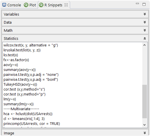
The snippets view offers several thematic ordered templates for the use in the expression textfield or the R editor. Context information is shown up if a template is selected. A double-click with the left mouse on the selected template transfers the text to the Expression textfield. A Right-Mouse (double-click) transfers the text to an opened R editor.
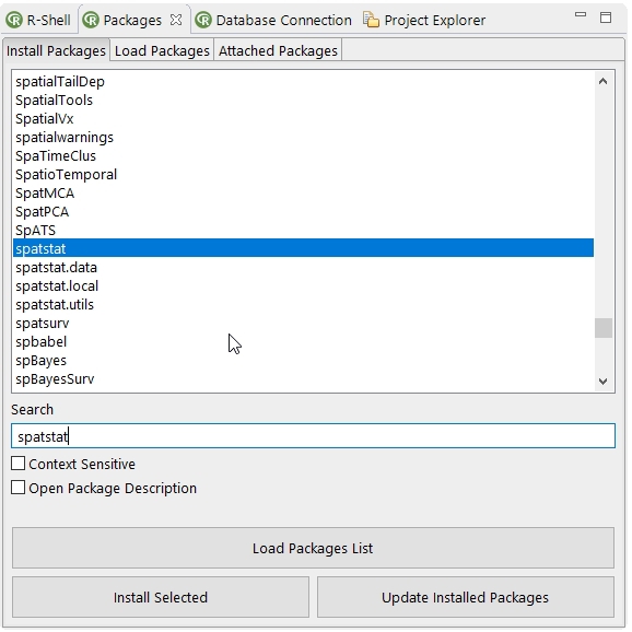
4.6.2.4 The Packages view
The packages view consists of three tabs to install, load and manage R packages. In the Install Packages tab a package list can be loaded from the default R mirror (see 4.6.2.12↓) with the Load Packages list action and installed with the Install Selected action. If something went wrong with the installation it can make sense to start Rserve in a OS shell to get more information about the installation process (see 4.6.2.12↓). To find the right R package some search facilities are available to find the package in the package list and to get some information about the package (select the Open Package Description option). With the Update Installed Packages action all currently installed R packages (except the Rserve package) will be updated if possible.
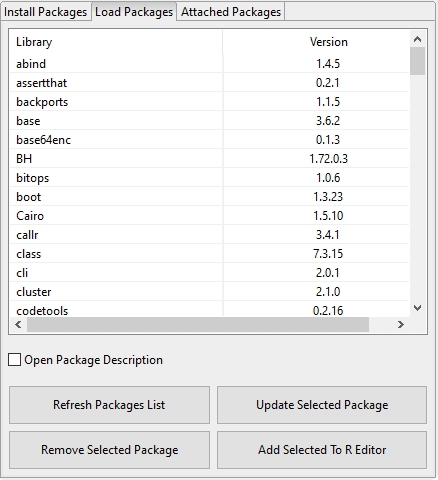
The Load Packages tab displays the currently installed R packages and their version numbers. This list can be refreshed with the Refresh Packages List action (a refresh of the list also occurs when the tab is switched!). A double-click on the list with the mouse loads the selected package which in turn also reloads the package code completion list for the R-Shell and the R editor. With the Remove Selected Package action a R package can be removed. With the Add selected to R editor action selected libraries can be added to an opened R editor as text (library(xxx)). With the Update selected Package action selected packages can be updated if an update is available. With the option Open Package Description a browser will be opened to display the current selected package information.
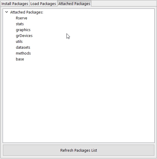
The Attached Packages tab displays the current loaded R packages. With the Refresh Packages List action this list can be updated (a refresh of the list also occurs when the tab is switched!). A context menu is available with an Detach action to detach a selected package and a Refresh packages list action.
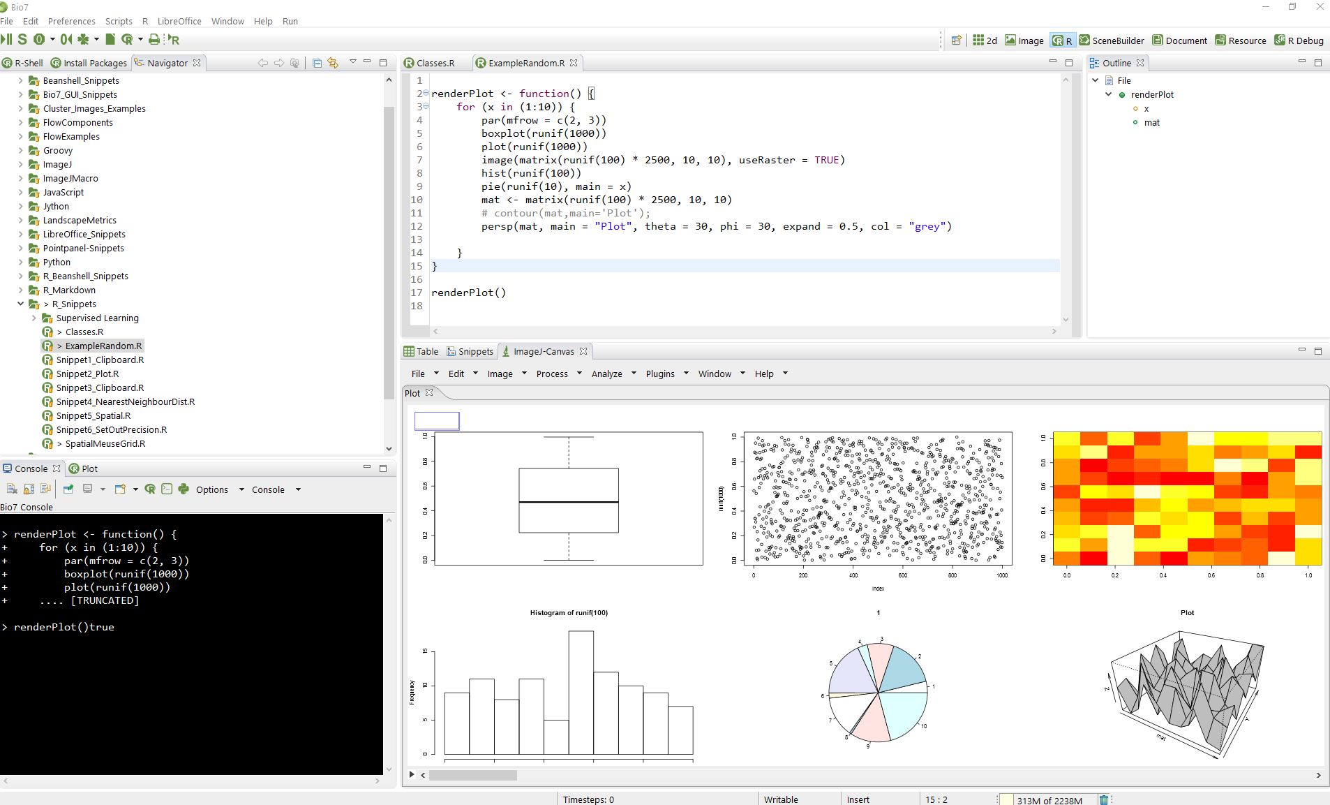
4.6.2.5 The Plot Data View
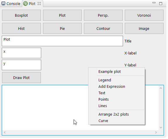
A selected data structure (in the data view of the Object tab) can be plotted easily with the different plot actions in this view. The selected plot type has to be appropriate for the selected datatype. Default all plots are created as an Image in ImageJ. If the option Detour is enabled all commands are transferred to the textfield for customization (templates are available in the context menu of the textfield). The customized command then can be plotted with the Draw Plot action.
4.6.2.6 The R Editor
The R editor of Bio7 supports the syntax of the R language. If an R file is created with the default wizard the extension of the created R script file is *r. If you have an *.r file outside the workbench, this file can simply be dropped to a project of Bio7. If a R file has been opened, the toolbar of the Bio7 application displays a new action item for the interpretation of R scripts (if a connection to the Rserver and R has been established).
The R editor of Bio7 is connected to an R parser. Each time the R code in the editor is changed the editor file is parsed and error or warning markers are created - visible as icons in the vertical ruler and underlined in the text where the errors or warnings have been detected. In addition the R parser creates code analytics to detect and inform about several flaws in the code. If some code assistence is available a light bulb will be displayed in the vertical ruler of the editor. A click on the quick fix icon opens a code suggestion which can be applied with a mouse click. The error and warning messages can also also opened if the underlined marked word is hovered. Hovered quick fixes can be confirmed with a mouse click, too.
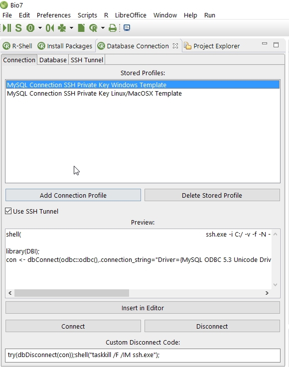
4.6.2.7 The Database View
The database view contains three tabs to configure a database connection. For a database connection the ODBC drivers have to be installed for the dedicated Operating System. The R packages odbc and DBI have to be installed, too. In the first tab Connection some templates are available which can be selected to be used for a custom connection and displays the connection information of the Database and SSH Tunnel tab.
- Install the ODBC drivers and R packages (odbc, DBI)
- Select one available default profile
- Update the login data on the Database and (if enabled) SSH Tunnel tab. In additon customize the Custom Disconnect Code for a live connection. Please note if no database password should be stored for the database connection leave the password field blank. For each live database connection a password dialog will be opened to ask for the username and password (handy if you don’t want to store the database password or the password should be hidden in a public area)
- Store the current profile with the Add Connection Profile action
- Use the Connect action to establish a database connection
- Use the Disconnect action to execute the R code given in the Custom Disconnect Code textfield
In the following section the different tabs and settings are described in detail.
- The Add Connection Profile action stores the current settings of the Database and SSH (if enabled) entries in a new profile and adds the selected name to the list of available Stored Profiles (saved as a XML file in Bio7).
- The Delete Stored Profile action deletes the current selected profile and removes the profile from the Stored Profiles list.
- The Use SSH Tunnel option adds the settings of the SSH Tunnel tab to the database tab settings which will be previewed in the Preview textfield.
- The Preview textfield shows the current settings of the database and SSH connection which can be stored as a database profile.
- The Insert in Editor action transfers the database connection code to the current opened editor.
- The Connect action establish a connection with the credentials given from the Database and SSH Tunnel tab. The connection is stored in the variable con
- The Disconnect action executes R code given in the textfield Custom Disconnect Code (available to control the SSH connection!)
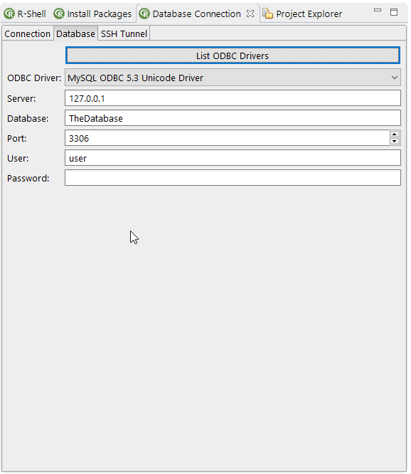
- The List ODBC Drivers action searches for available ODBC drivers on the OS and add them to the ODBC Driver list
- The ODBC Driver list let you select a ODBC driver for a database connection by name found by the action List ODBC Drivers
- The Server textfield to enter the server address of the database
- The Database textfield to enter the database name of the connection
- The Port to enter the port of the database
- The User textfield to enter the username.If empty a login dialog will automatically be opened for the username and password
- The Password textfield to enter the password of the database connection. If empty a login dialog will automatically be opened to enter the username and password
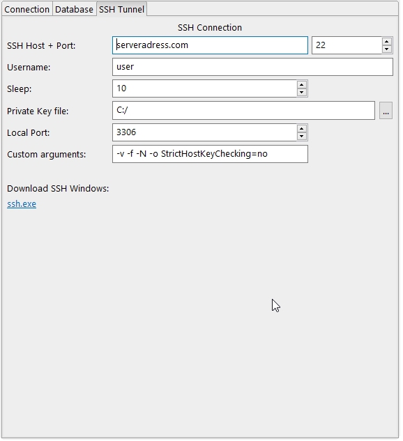
- The SSH Host textfield and Port spinner for the server address and port of the SSH connection
- The Username of the SSH connection (password should be stored in the SSH key!)
- The Sleep spinner to execute the sleep command on the remote server (default to 10s)
- The Private Key file textfield and file dialog action to set the location of the private SSH key
- The Local Port to set the port for port forwarding (This setting lets you specify a local port that will be forwarded to your remote host and remote port)
- The Custom arguments textfield to change or add custom SSH client options
4.6.2.8 Plotting
Since Bio7 1.7.1 it is possible to plot single and multiple plots with ImageJ as the default R plot device. Multiple plots are displayed in an ImageJ image stack (with the available slider you can select one plot in the stack). Plots and plot stacks can be saved as images and movies with ImageJ in different formats (e.g. stacks can be stored as *.avi or animated *.gif). The size of the plots and the format can be changed in the Rserve Plot Preferences of Bio7 (see 4.6.2.10↓) .
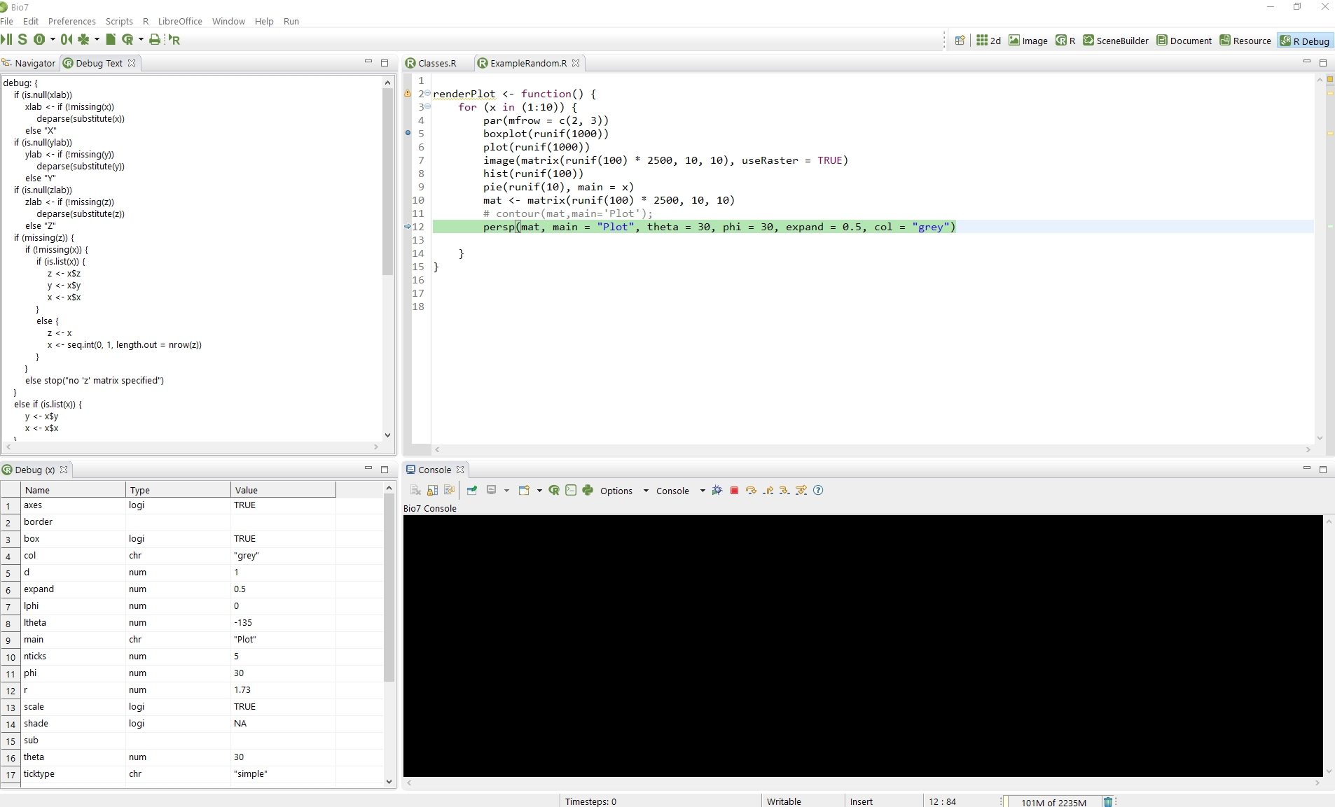
4.6.2.9 R Debugging Interface
Since Bio7 2.0 a debugging GUI for R is integrated as part of the R editor. To debug a R script a breakpoint has to be set inside a R function. If a breakpoint is set several actions are added to the default Bio7 console. For the debugging process the native R console has to be started (The Rserve connection will be automatically change to the native mode if alive!). To start a debugging process the “Debug Trace Action” has to be invoked and the traced function has to be executed in the R shell (see screenshot below). In the shell several debugging actions are available:
- The Debug Trace Action to start the debugging process.
- The Stop action to stop the debugging process.
- The Next action to go to the next statement.
- The Continue action which continues with the execution without single stepping.
- The Step Into action to step into function calls.
- The Finish action to finish the current loop or function.
- A Help action to display R debugging console commands.
- Set a breakpoint.
- Set a conditional breakpoint - Syntax e.g. : if (x==5) browser() which is a wrapper for: trace(fun, quote(if (x == 5) browser())).
- Edit a conditional breakpoint.
- Delete a selected breakpoint.
- Delete all breakpoints.
4.6.2.10 R Plot Preferences
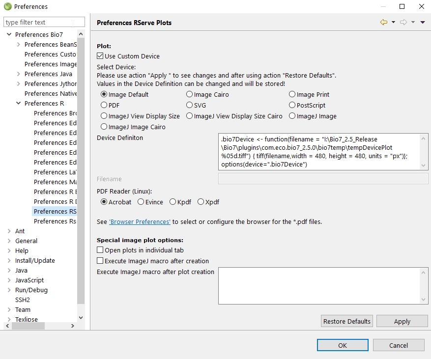
In the preferences several options are available to adjust the R plots. The default plot size can be changed in the textfield Device Definition (or the whole plot definition). Beside the option to plot images in ImageJ it is possible to open plots in different applications. Some templates in the preferences can be selected to switch e.g. to a *.pdf (multiple plots can be displayed) or *.svg plot (displaying a single plot) which will be opened with the default registered software if available – for *.svg i recommend http://www.inkscape.org to improve the plot appearance). Antialiased image plots can be enabled with the Image Cairo option. To change the default Device Definition in the textfield press the action Apply. With the Special image plot options plots can be opened in individual image tabs or macros can be excuted after image creation (handy if you automatically want to scale images after plot creation). Please note that the preferences will be saved if you press the OK or Apply button.
4.6.2.11 Help
As noted earlier if a command has been typed in the textfield of the R-Shell view and the ? button has been pressed the action tries to open the default help page for the command in the Bio7 browser (same as typing ?+command in R).
4.6.2.12 Rserve preferences
There are several Rserve preferences available wich are described in this section.The following preferences can be adjusted:
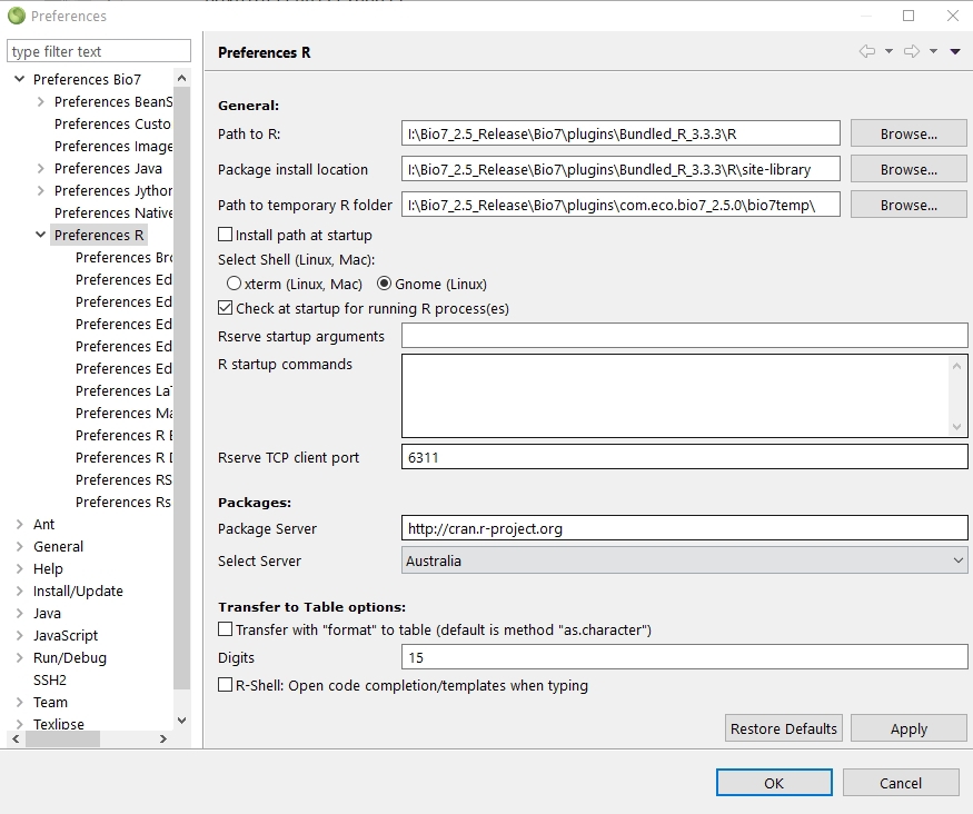
(1) General
- The path to the R install location.
- The default package install location.
- The Path to temporary R folder options sets the path to the Bio7 R temp folder. In the temp. folder some plot images and R files are temporarily stored.
- The Install path at startup option installs a registry path to R in the Windows registry (deprecated).
- The option Check at startup for running R process(es) warns for running R processes which can interfer a newly started R/Rserve native process.
- The Rserve startup arguments can be adjusted to start Rserve with custom arguments.
- The R startup arguments can be adjusted to start R with arguments when started together with Rserve.
- The Rserve TCP client port option configures the running Rserve client port of the rserve application.
(2) In the Packages preferences you can select the default R package mirror to download R packages from. In addition you can set the install location of the packages.
(3) In the Transfer to Table options the transfer method to the Bio7 Table from R can be specified to adjust the numerical precision of numbers. Please consult the R documentation for the command format.
(4) The option R-Shell:... enables the automatic code completion of the R-Shell view (restart of Bio7 necessary!).
4.6.2.13 R Editor
For a description of the R editor see 4.6.2.6↑.
4.6.2.14 Native R Excution
In Bio7 it is possible to execute R scripts and R commands without Rserve (10.1↓). In the Bio7 console an independant R console can be started which pipes commands directly to an instance of R. If the editor should be used with the native communication this has to be selected in the R preferences of Bio7. Some commands and GUI interfaces cannot be used if the native execution is selected
4.6.2.15 Create R Packages
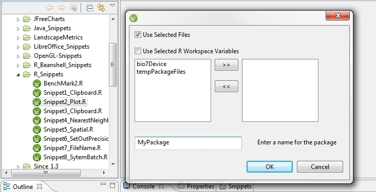
If R files are selected in the Navigator view an action is available which opens a dialog to create a R package skeleton from files or selected R workspace variables. After the creation if the created R package folder is selected several available actions help in the build process of a package.
- Build PDF From .Rd to create PDF documentation of *.Rd files.
- Check R Package - To check if the package is properly configured.
- Build R Package - to start the build process of the package
- Install R Package - to install the R package.
4.6.2.16 Create R Packages with the devtools package.
Since Bio7 2.5 a new way of creating packages have been added to the context menu of the Navigator view by using the devtools library (https://github.com/hadley/devtools) to create, test, compile and distribute a new R package. To setup a new R package create a project folder in the workspace of Bio7 and then select the folder and execute the “setup” action in the context menu of the Navigator view. Documentation will be created if roxygen comments have been added to the R scripts by executing the “Document” action.
- Setup - Setup R package in (project) folder (devtools)
- Load All - Simulates installing and reloading (devtools)
- Document - Updates the documentation, etc. (devtools)
- Test - Tests the packages (devtools)
- Install - Installs the packages
- Build - Builds the packages
- Check - Checks the packages
- Build Windows - Builds the package on Windows
- Run Examples - Runs all examples of the package
- Check Manuals - Checks all manuals
- Release - Releases the package
For some of the listed actions above the OS pseudo terminal in the console view has to be activated or will be activated. Custom flags can be added in the R Preferences Built Tools of Bio7. Please note: For the built process of R package binaries some extra tools are needed (especially for Windows). Please consult the R instructions (http://cran.r-project.org/doc/manuals/R-exts.html) on the internet or search for available tutorials. For tests on the Windows OS I installed a Latex environment (MiKe\SpecialChar TeX with inconsolata.sty style file installed) and the Rtools distribution for Windows (http://cran.r-project.org/bin/windows/Rtools/).
4.7 Document Perspective
A special document perspective is available which opens a rendered document (HTML, PDF, etc.) side by side with a Bio7 editor (e.g., markdown, latex, HTML). The editor in this perpspective is shown by default.
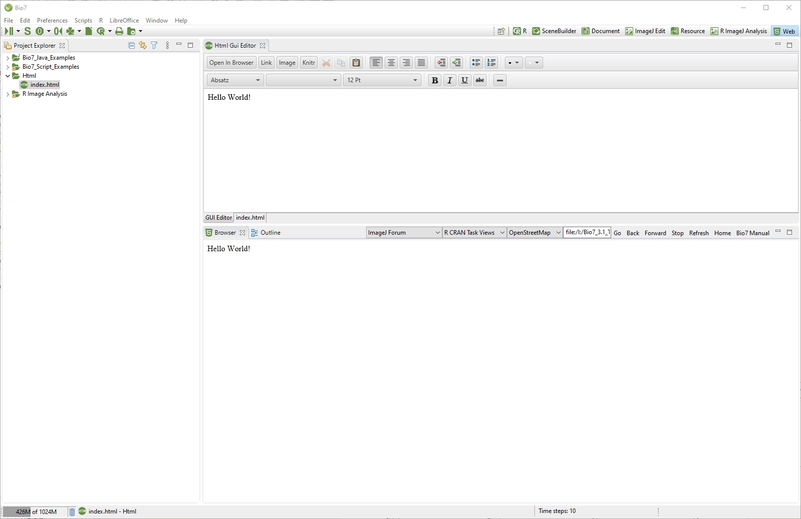
4.8 The HTML Perspective
The HTML perspective is a special perspective to create websites with the HTML editor of Bio7. The HTML editor will be opened if a *.html file is selected or created. It contains two tabs to switch between the source editor and a text interface based on JavaFX. Projects are stored and displayed in the Navigator view (left) which is also displayed by default in this perspective. You can use the Bio7 file wizard to create a new *.html site. With the Open In Browser action the created content can be displayed in the default browser of the OS (embedded as a Browser view below the editor).
4.9 The 2d Perspective (hidden by default)
The 2d-perspective offers several views for displaying and adjusting simulations of spatial discrete models and spatial discrete individual based models.
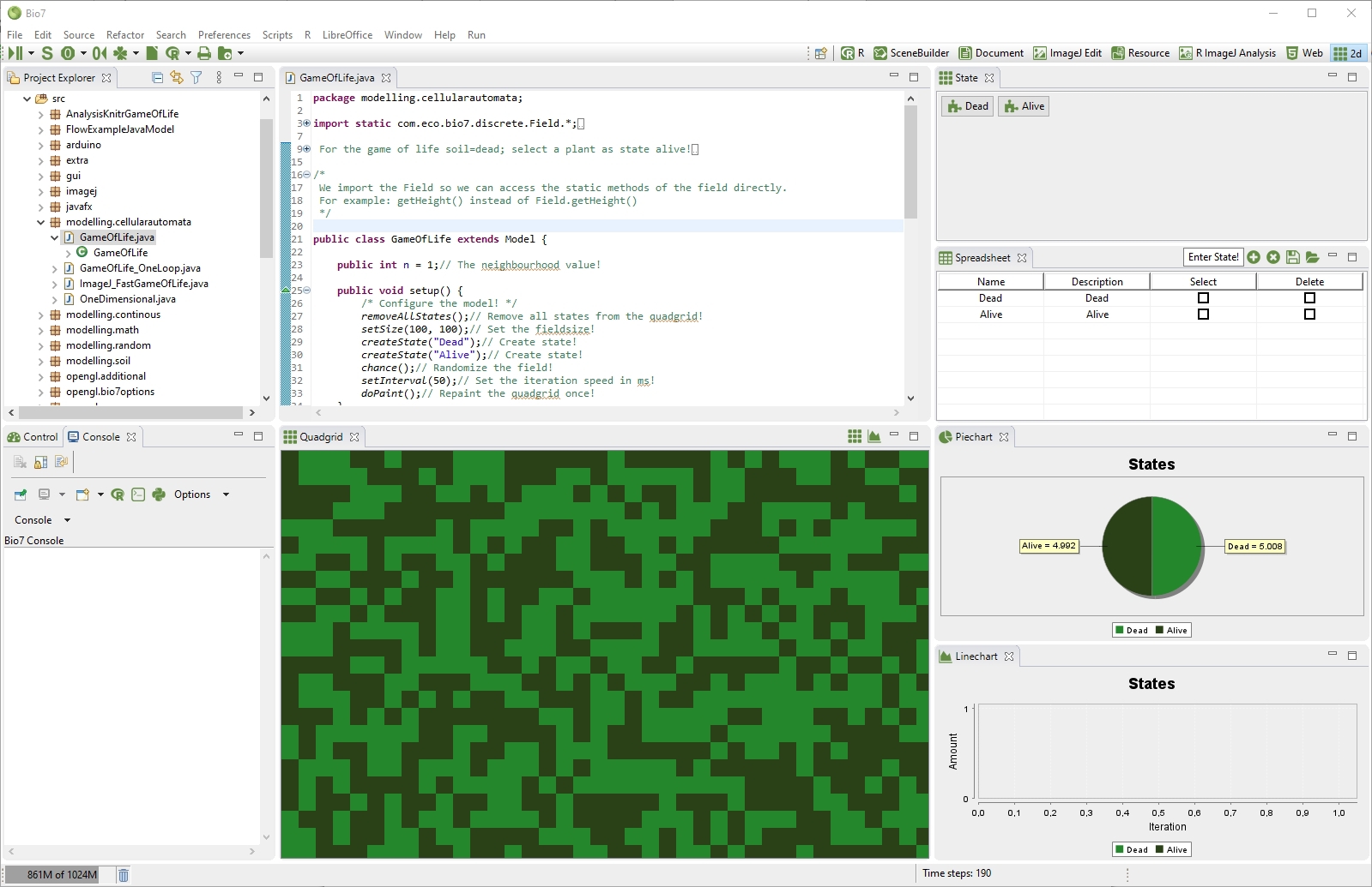
4.9.1 The Quadgrid
The Quadgrid view (1) - like the by default hidden Hexgrid panel - visualizes a simulation field for discrete simulation models. At startup only one state with value 0 is dispersed in the Quadgrid (respectively Hexgrid) field. The panel itself is a visualization of states stored in an two dimensional integer array. In the grid array (xystate) numeric states of type integer are stored for simulation purposes. By default there is also a temporary array available (xytempstate) for an intermediate store of states when calculating patterns for the next timestep (t+1) as it is usual in grid based modelling. The arrays can be accessed by means of a small API to facilitate the development of such models. In the panel it is possible to zoom in or zoom out with the scroll wheel of the mouse. The state of the cells can be adjusted by clicking and dragging on them. With a right click on the Quadgrid panel a context menu opens with the possibility to select states in the Quadgrid panel (Keys: Alt+S).
1/*A simple example to show how to produce and set random cells!*/ 2 3int rand; // A random number variable! 4 5public void run() { 6 for (int y = 0; y < Field.getHeight(); y++) { 7 8 for (int x = 0; x < Field.getWidth(); x++) { 9 rand = (int) (Math.random() * Bio7State.getStateSize()); 10 Field.setState(x,y,rand); 11 Field.setTempState(x,y,rand); 12 13 } 14 } 15 16}
Figure 4.52 Java example to update the states of the Quadgrid
4.9.1.1 Transfer Quadgrid Data and Patterns to R
In the toolbar of the Quadgrid view population and pattern data can be transferred directly to R with two available actions.
- Transfer of population counts: The first action transfers population counts of all current states to R. The counts can be deleted in the toolbar with the Counter Reset action (see 4.9.5↓).
- Transfer of pattern: The second action transfers the current state pattern as a matrix to R.
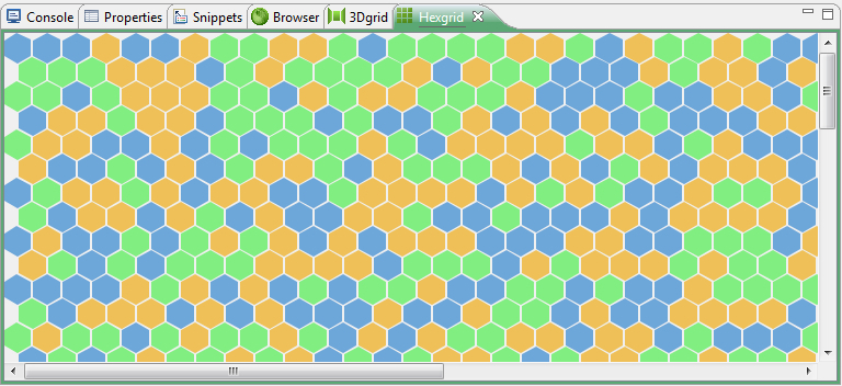
4.9.2 The Hexgrid
It has sometimes advantages to create hexagonal designs in experimental setups which will reproduce a binned pattern more naturally instead of the Quadgrid. A central cell in a Hexgrid is surrounded by six neighbours. All have the same euclidean distance from the centre to the surrounding cell. Bio7 offers a hexagonal grid which is by default hidden, but can easily be activated with Window\SpecialChar menuseparatorShow View\SpecialChar menuseparatorOther\SpecialChar menuseparatorBio7-Panels\SpecialChar menuseparatorHexgrid
4.9.3 Randomize the Quadgrid (Hexgrid)
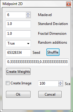
In the Bio7 toolbar a special dialog can be opened to create a pattern with the Midpoint Algorithm (see [6]). The Midpoint Algorithm is especially suited for creating clustered random patterns like landscapes and super individuals (e.g. clumbed vegetation patterns which grow in a colony like e.g. moos).
- Maxlevel (maxlevel) adjusts the maximal number of recursions. The default action creates a 2 Maxlevel* 2 Maxlevel grid pattern from activated states (integers) in the quadgrid.
- Standard deviation (sigma) adds the intial standard deviation.
- Fractal dimension (H) this parameter determines the fractal dimension (D = 3 - H)
- Random additions (addition) turns random additions on/off.
- Seed (seed) adjusts the seed value for the random number generator (the action Shuffle creates a random number)
- With the Create Weights action state changes (if changed in the quadgrid) are considered and the amount of weights are set with equal proportions in the textfield. It is possible to change the value (proportion in the Quadgrid) for each state in the textfield individually.
- The Create Image option can be selected to create a random pattern with float numbers in ImageJ (e.g. for a height map or continous clumbed nutrient matrix). The default values can be multiplied with a scale factor in the Scale box.
4.9.4 The Linechart and the Piechart
The Linechart and the Piechart views (3) serve as a monitor to watch population size and count the different states in a simulation run. Regardless how fast a simulation runs the charts get updated every second. With a right-click on the charts several options are available. For example to store an image of the chart or to adjust some chart parameters. The Piechart visualizes the count of the activated states inside the Quadgrid (Hexgrid). The Linechart displays the amount of states in dependence of the simulation steps. When a simulation is started coloured lines will visualize the amount of states over the time. The colours of the charts will be automatically updated when the colours are changed in the Plants view.
4.9.5 Recording the Amount of States over Time
In Bio7 a list is available which stores the values of a simulation run. Each state amount in every timestep is automatically recorded. With the Reset action (see 3.1.10.1↑) in the toolbar this values can be deleted for a new run starting at timestep 0. In addition it is possibly to delete the values programmatically. If you don’t need this feature you can deactivate it in the Bio7 preferences.
4.9.6 The Time and Space Control
When the Time&Space (4) item is enrolled (by default it is!) a panel appears showing information about the time steps a simulation has proceeded. Additionally every time step is displayed as a month and 12 time steps are displayed as a year. Furthermore several sliders for the adjustment of the parameters calculation speed (time resolution) and field size (capacity) are available. Additionally a checkbox and a button are displayed which enable the resize event after a slider change.
- The first slider (Speed) is responsible for the calculation speed of the calculation thread. It can be set to values from 10-1000 units.
- The visible sliders below (Fieldsize) can be moved to values from 1 to 2000. They are responsible to adjust the field size of the different grids in Bio7 (Quadgrid, Hexgrid) The maximum field size which can be adjusted in Bio7 is a field size of 2000*2000. When moving the sliders for the field size several views will be updated instantly. TheQuadgrid panel will be updated when a resize event takes place (the Hexgrid panel and the visualization of 3d panel only if opened). After resizing the new indexes (2d grid array) are instantly accessible (e.g. programmatically).
- When the checkbox Resize after adjust is activated the resizing takes place after the button Resize has been pushed. This is recommended when the field size is >400 because the resizing then is done in one call. Info: The speed of a resize event is also dependant on the amount of grid panels which are currently visible in the Bio7 window (e.g. Quadgrid, Hexgrid or 3d panel!).
4.9.7 Spreadsheet
In the top-right of the perspective the Spreadsheet view (5) offers a visualization of states. The name and the info are displayed by default. Also two columns with check boxes are displayed. By enabling a check box in the column “Select” a state can be selected to set (draw) a specific cell in the quadgrid. With the checkbox in the column “Delete” states can be selected for deletion.
4.9.7.1 Spreadsheet Toolbar
In the spreadsheet toolbar (6) the pattern and adjustments (height, width, amount of states) of the quadgrid can be saved to a file. It is also possible to store the current Java source with the pattern and adjustments. This simulation file can be reopened with the open action or simply dragged on the general toolbar of Bio7. If Java source is detected in a simulation file it will be compiled and loaded and if available the setup method will be executed. In addition the following toolbar actions are available:
- With the toolbar textfield new states can be defined (press the + button or press Return).
- Selected states in the “Delete” column can be deleted with the “Delete” action.
- If a state in the spreadsheet is selected the state can be set in the quadgrid (via the mouse device - click or drag).
4.9.8 File Storage of Patterns
As already mentioned a grid pattern can be stored (optionally along with the Java model source) with the save action in the toolbar of the spreadsheet.
4.9.8.1 The State View
In the state view (7) the different states are displayed. With the state button(s) the default color of the states can be changed easily.
4.10 Custom Perspective, Views and Menus
It is also possible to fill an available custom perspective (“Custom”) with Bio7. All views from the application can be used to layout the perspective for certain tasks.
4.10.1 Custom Views
Besides the possibility to extend Bio7 with custom perspectives also multiple custom-views can be defined for embedding self defined GUI’s in Bio7. Self defined JPanels (Swing), SWT canvas and Draw2d panels can easily be embedded in a Custom Controls view. Multiple custom views can be created with a unique id.
4.10.2 Custom Menus
Another nice feature of Bio7 is the simple way to extend the Script menus in Bio7 with BeanShell, Groovy, Jython scripts, R scripts and ImageJ macros. Bio7 recognizes files dropped to special folders automatically and extends the menus with the filename of the dropped files. for an overview see (see ↓.
4.10.3 Custom Startup
Groovy scripts can be used to customize the platform directly behind the start of the Bio7 application. These scripts will be executed with the Groovy interpreter. The scripts have to be placed in a specialized folder (↓) for custom activities like :
- BeanShell, Groovy, Jython, R, JavaScript, ImageJ customizations or imports at startup.
- Open or close a custom perspective or a view.
- Execute a startup setup in the different panels.
- Invoke an action from the Bio7 platform.
- Import libraries.
- Start a server application at startup.
5 The Editors of Bio7
5.1 General Features
There are several editors integrated in Bio7 which support the syntax of different programming languages and a specialized Flow editor to drop files from the other editors for execution. The "language" editors support the syntax of the languages Java, BeanShell,Groovy, Jython and R. A text editor is also offered by default integrated in the platform (an editor for arbitrary files as well!). All editors if opened offer more or less customized menus and toolbars and also offer custom context menus for the work with the different languages. By activating a language editor, typical text tools are activated in the edit menu of the main menubar of the Bio7 application. Some creation notes are listed below.
- Before creating a file, a Project has to be created where the files can be placed (File ▷ New ▷ General ▷ Project).
- A file can be created by using a wizard, which can be activated in the File menu. (File ▷ New ▷ Other ▷ xxx) or in the context menu of the Navigator. (e.g.: New ▷ Other ▷ xxx).
- The file itself will be opened in the editor area, which can be hidden or shown in a perspective by selecting the action Window ▷ Show/Hide Editor.
5.1.1 Editor Code Templates
Alternatively to the simple Snippets view (see ↓) all language editors offer code templates by pressing the key combination Ctrl+Space (see below). Eventually the key settings have to be changed depending on the OS!
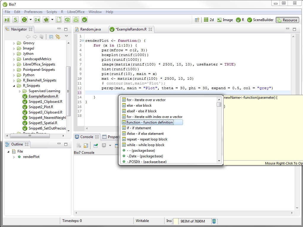
Templates for the Bio7 editors can be created and stored in the preferences dialog (Preferences ▷ Preferences Bio7 ▷ Preferences xxx-Editor ▷ Template Editor xxx).
For a detailed description of the Code Templates see: http://help.eclipse.org/kepler/index.jsp?topic=%2Forg.eclipse.jdt.doc.user%2FgettingStarted%2Fqs-EditorTemplates.htm
By default it is possible to share this self defined code templates with others by using the integrated import/export functions of the different template editors available for each language in Bio7.
5.1.2 Preferences of the Editors
In the preferences dialog of Bio7 there are a lot of functions available to customize the different language editors. For example, the fonts for all editors can be customized under General ▷ Appearance ▷ Colours and Fonts. If the colours of the keywords, etc. should be changed, it could be done under Preferences Bio7 ▷ Preferences xxx-Editor for a selected editor.
5.1.3 The R Editor
Bio7 contains a R editor which is described in the R perspective section (see 4.6↑).
5.1.4 R Markdown Editor
Since Bio7 2.3 it is possible to write R markdown documents with the help of the rmarkdown package https://cran.r-project.org/web/packages/rmarkdown/index.html. A simple markdown editor is available by default in Bio7 with helps in the creation of rmarkdown supported document types. A wizard in the file menu is available, too to help in the creation of a default rmarkdown document export type.
5.1.5 LaTeX Editor
The Texlipse editor http://texlipse.sourceforge.net/ integrated in Bio7 can be used to create LaTeX and LaTeX knitr documents. For a complete manual see: http://texlipse.sourceforge.net/manual/. If the editor is opened with a *.Rtex knitr file an action will be available to compile the document to a valid *.tex file eventually with embedded R commands and plots.
5.1.6 HTML Editor
The HTML editor of Bio7 embedded, e.g., in the HTML perspective (see 4.8↑) is a graphical and text based editor (multi page) for the creation of pure HTML and rmarkdown HTML files.If the editor is opened with a *.Rhtml knitr file an action will be available to compile the document to a valid *.html file eventually with embedded R commands and plots.
5.1.7 Java
Since Bio7 2.0 the JDT Java editor is used to edit Java source files. A description of the JDT editor can be found on the Eclipse documentation website http://help.eclipse.org/luna or in the Bio7 help.
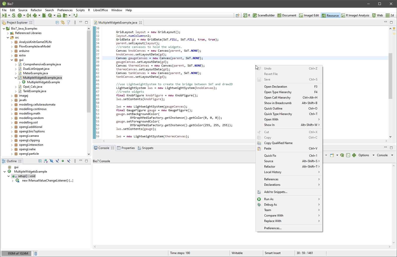
5.1.7.1 Since Bio7 1.7.1 Full Class and Multiple Class Compilation is Supported!
In the Java preferences of Bio7 you can switch between full class and classbody compilation - deprecated in Bio7 2.0 - (1). In addition it is possible to adjust some compiler properties.
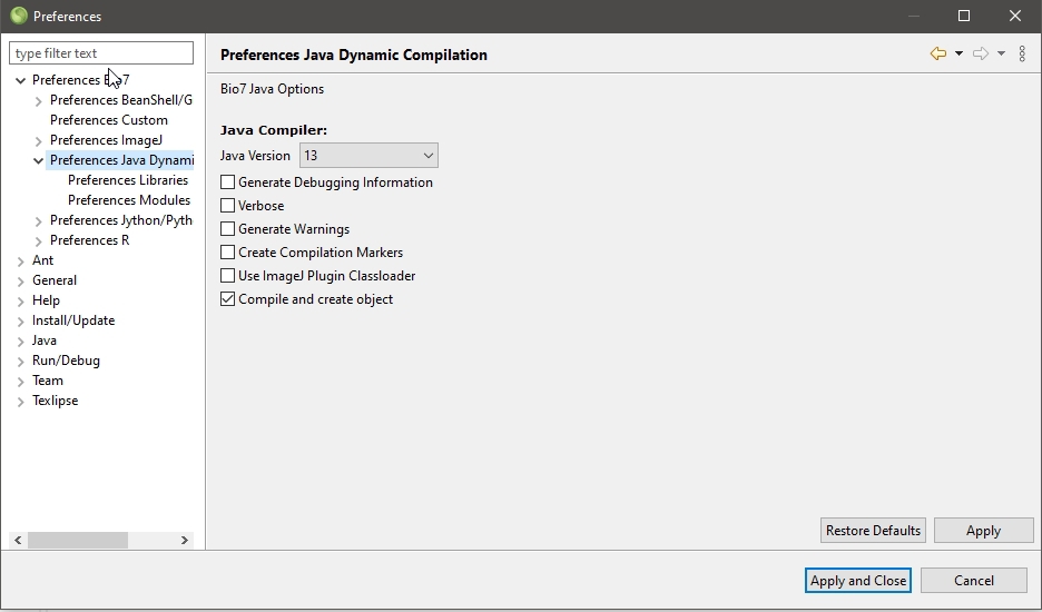
5.1.8 BeanShell and Groovy
The BeanShell/Groovy editor as well as the Java editor supports the Java syntax. Code templates, (identically to that in the Java editor) are available, too (some script code templates may differ!). In general BeanShell or Groovy are capable to interpret ordinary Java code but also have complete scripting capabilities to facilitate the development process of programming. Scripting code as well as Java code can be executed with the actions which are shown in the toolbar.
The reasons that BeanShell, Groovy and a separate Java compiler have been added to Bio7 are the following:
- Need for speed in complex applications: The embedded Java compiler compiles the Java code to bytecode while the interpreted languages interpret the code which is much slower and sometimes is not sufficient for resource intensive calculations (though compiled code will be executed also very efficiently by BeanShell, Groovy or Jython!). However new versions of the different interpreters close this speed gap more and more.
- Scripting capabilities: With BeanShell, Groovy (and Jython) it is possible to create highly dynamic applications with customized scripts. Script templates like the snippets can easily be recycled for custom modifications. Scripts can be used to extend the Bio7 Script menus.
- Direct interaction: With the BeanShell, Groovy (or Jython) console you can interact directly with the methods and integrated API’s of Bio7.
Code, which was written for the Java compiler can easily be switched to BeanShell (supports full Java syntax up to version 1.4!) or Groovy (minor differences).
The default imports for the BeanShell, Groovy and Jython interpreter can be changed in the file ...\plugins\com.eco.bio7_x.x.x\bin\imports\xxxxx.properties (Windows)
5.1.8.1 Special Actions in the Context Menu of the Java and BeanShell/Groovy Editor
The context menu of the BeanShell/Groovy editor and the Java editor offers some methods for editing the source and for source conversions. These are (beside the regular actions of the platform):
- Add Block Comment: Surrounds the selected code with a block comment.
- Remove Block Comment: Removes a selected block comment. (A precise selection is necessary!).
- Format Java: Formats regular Java code (To work with BeanShell or Groovy please create Java code inside the BeanShell/Groovy editor!).
- Format selected Java: Formats only the selected code. This is sometimes necessary if the formatter can not format the entire code.
- R Source Conversion: Converts Rscript code. This converter helps to convert R expressions for the use e.g. in an BeanShell or Groovy script using the Rserve API.
5.1.9 The Python/Jython Editor
A Python/Jython editor is available to execute Python/Jython scripts. The Bio7 API can be used with Python/Jython, too. The editor comes with typical editor actions similiar to those which were already described for the other language editors.
1# A Jython example which overrides the run method 2# of the inherited Model class of Bio7! 3# The method run can be called from the Start/Pause action 4# of the Bio7 toolbar! 5 6class jythonClass(Model): 7 8def run(self): 9#print index 10Field.chance(); 11Field.doPaint(); 12 13#We instantiate the class! 14model = jythonClass() 15#We set the class as the compiled class! 16Compiled.setModel(model);
Table 5.1 Jython example which uses the Bio7 API
5.1.9.1 Native Python Execution
It is also possible to execute Python scripts with the Jython editor if the native execution is enabled in the Native preferences of Bio7 (see: 10.1↓). If the Python package “Py4J” is installed ( http://py4j.sourceforge.net/) in the Python distribution the Bio7 API and Java libs can be acessed from within CPython (see 5.2↓). Therefore the Java Py4J Server has to be started in the scripts menu of Bio7 (which is momentarily by default available in the Linux and Mac version of Bio7 2.0). Note: It is also possible to install the popular “PyDev” Python editor ( http://pydev.org/) into Bio7 and execute the opened Python scripts (you have to open them with the PyDev editor) with the available Bio7 action in the main toolbar. The available Bio7 action cares about the execution of the script in the Bio7 Python/Jython environment and console.
1# A Python Py4J example which transfers values 2# from the ImageJ Results table and plots them with 3# the Matplot lib. 4# For this example Py4J has to be installed in Python 5# and the Py4J Server has to be started! 6 7import numpy as np 8import matplotlib.pyplot as plt 9from py4j.java_gateway import JavaGateway 10from py4j.java_collections import JavaArray 11 12gateway = JavaGateway() 13results=gateway.jvm.ij.measure.ResultsTable 14analyzer=gateway.jvm.ij.plugin.filter.Analyzer 15 16#get the results from the Java ImageJ API! 17rt=analyzer.getResultsTable() 18res=rt.getColumn(0) 19lastCol=rt.getLastColumn(); 20 21values=[[0 for x in range(len(res))] for x in range(lastCol+1)] 22for x in range (0,lastCol+1): 23 vals=rt.getColumnAsDoubles(x) 24 if (isinstance(vals,JavaArray)): 25 print (’’) 26 for y in range (0,len(res)): 27 values[x][y]=vals[y] 28 29#Plot the values! 30plt.boxplot(values) 31plt.show()
Table 5.2 CPython Py4J example which uses the Java ImageJ API
5.1.10 The ImageJ Macro Editor
Bio7 embedds a complete ImageJ macro editor with dynamic error detection, syntax highlightening, code completion, formatiing features, debugging interface, etc.
In the ImageJ Edit perspective several views are arranged to support the creation and execution of ImageJ Macro files. A special debugging interface is available in the Debug view.
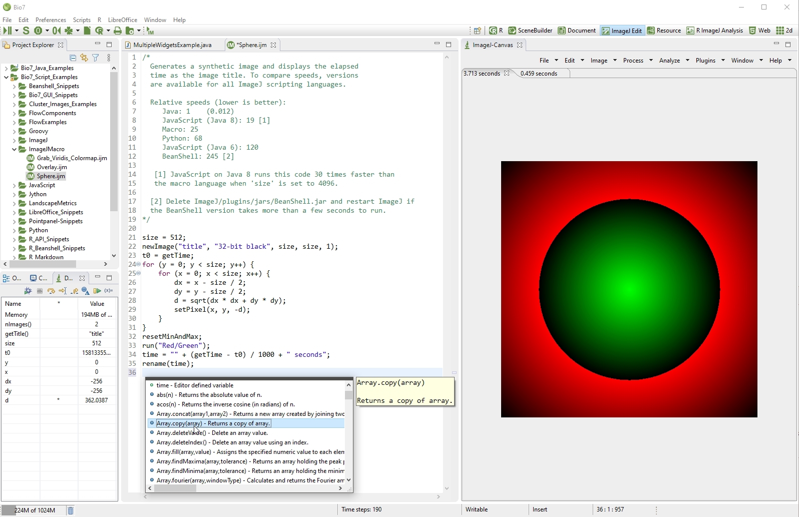
5.1.5 The Flow Editor
The Flow editor of the Bio7 application is capable to handle and execute different files by their extension and display and arrange them in a flowchart like structure.The Flow editor is useful to:
- It can be used to create complex sensitivity analysis for created models
- It can serve as a guide for complex analysis of all tools offered by Bio7.
- Or it simply can be used to visualize complex workflows.
The main strength of this tool is that you can assemble all methods and information, created by files for modeling, statistical analysis or image analysis in a profound analysis. The Flow editor of Bio7 helps to organize and visualize the creation and analysis of ecological models. A flowchart by definition is a graphic representation of a sequence of operations.
If the editor is opened default actions will be added to the Bio7 toolbar (1) and a new menu will appear in the menubar of the application. Additionally, a specialized context menu will be available for calling different methods inside the Flow editor. In the flowchart of Bio7 files can simply be dragged from the Navigator view (2) of Bio7 and dropped into the Flow editor (3) of the application. According to their file extension these files are executed in the sequence of the flow which has been created. A created Flow editor file has the extension *.ecoflow. Some other files will be handled by default from the Flow editor when they are dragged from outside the workspace. Executable files (*.exe) will be executed, too and it is also possible to execute these files with an argument (by creating a file with the extension *.argument). Files from external that have different extensions will be executed according to their registration in the system environment. Furthermore an Outline view (4) on the left will show an overview of the flow - if the flow cannot easily be displayed in the main window because of its size a blue rectangle will be displayed in the Outline for a flow selection. The selection is the area of the flow which can be displayed in the main Flow editor window. A new Palette bar (5) will also be displayed for inserting flowchart elements in a newly created file.
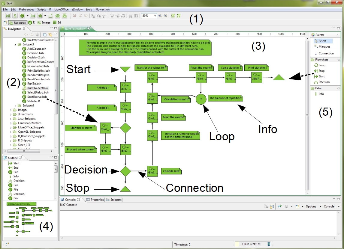
5.1.10.1 Execute and Verify a Flow
The execution of a flow will be triggered with the item FlowAction in the top-right of the toolbar (1). In addition since Bio7 1.5 a new action - left action - is available to verify the connections for a valid Bio7 flow graph.
5.1.10.2 The Palette of the Flow Editor
For the creation of a running flowchart it is necessary to create a start and a stop element in the flowchart. By activating an element in the Palette these elements can be placed anywhere in the flowchart with the mouse at the appropriate coordinates (pressing mouse button will drop the component). Additionally when an element has been placed in the flow it can be dragged to any coordinates in the flow panel. All other elements in the Palette can be placed by this procedure too. The following elements are available and their values can be adjusted in the Properties view. Furthermore some properties can be changed directly in the shape (mouse click on the element) The following elements are available:
- Start : The start of the flow - necessary for execution !
- Stop : The end of the flow - necessary for execution !
- Loop : A loop will repeat a sequence in the flowchart. The number of iterations can be adjusted with an integer value directly in the shape (click and hold ca. one second to edit).
- Decision : A decision in the flow will execute an if statement. According to a self defined condition a static variable (Bio7Flow.setDecision(“true”)) can be set to true or false. The direction of the flow then depends on the linked connection which can be set to true or false in the properties dialog (select the connections to set the values).
- Info : A single line label for an info which can be edited in the shape.
- Connection: To determine the sequence of the flow Connections are available to connect components. If selected in the Palette directed connections can be drawn from component to component.
- Selections can be made with the Marquee tool and the Select tool (multiple selections are possible).
There are several tools available for adjusting the components and the layout of the flow. In the toolbar of Bio7 several items will be enabled when components are selected alone or in a group. By default the zoom action and the flow action are enabled.
- With the Zoom In, Out actions it is possible to zoom in or to zoom out in the flow (by using the combo box or the lens items). If an opened flow was changed, the toolbar items for undo and redo could be used to undo or redo changes in the flow.
- Furthermore components can be deleted with the Delete item and so removed from the flow (or by pressing the delete key).
- If more than one component is selected the alignment actions (Align Width, etc.) and the Match Width/Height actions will be available to align shapes to the first selected shape or adjust the width or the height of selected shapes to the properties of the first selected component.
- Additionally the added menu Flowaction in the menubar of Bio7 offers three further options for the alignment and layout of the components.
- When the option Rulers is selected and marked rulers in the flow will be made visible for the exact layout of the flow components. By dragging horizontal and vertical lines from the ruler (like it is known from image software) components can easily be aligned to the visible ruler lines. The alignment will be supported by artificial lines (red lines) which occur when the alignment criteria are met.
- The option Grid will enable a grid in the flow. When enabled, the components can be arranged in discrete coordinate steps according to the default grid size in the flow. Furthermore artificial lines will occur (green lines) with the enabled option Snap to Geometry when a translated component matches the alignment of another component in the flow. The grid size can be adjusted in the context menu of the Flow editor.
The context menu offers some of the aforementioned methods and several new methods. The new methods are:
-
The options Manhatten Router and Shortest Path action are responsible for the layout of the connections.
- The Shortest Path action applies the shortest path algorithm to find paths around obstacles in the flow.
- The Manhatten Router algorithm will use rectangular lines for connections in the flow.
- The Save action will save the current flow to the before defined file (Save as in the Bio7 main menu available!).
- The Save Image action will save an image in the formats *.gif*, *.jpeg, *.ico to a file. The current size of the flow will determine the pic size (the rulers display the size of the flow in pixel. So be cautious not to store large images with a resized flow !).
- The Debug Mode option enables a visualization of the current flow by colouring the active shape white to mark files that are currently interpreted or compiled, etc. A mouse-click on the flow deletes marked components.
- Size Layout Grid opens a dialog to resize the grid (layout) if enabled.
If a shape or a connection is activated the properties of the component or the connection can be adjusted in the Properties view. This view is activated by default below the Flow editor or can be activated with the Windows ▷ Show View menu action. The properties dialog will only be necessary if you want create a decision inside a flow. All other component attributes are adjustable with the mouse. The following properties are displayed and can be adjusted:
-
The File/Loop/Info/Condition property displays the following attributes in dependence of the selected component:
- The filepath of a dropped component (relative path in the workspace. This path will be used for execution!)
- The amount of loops which should be made when the loop component has been selected.
- An info text if the info component has been selected.
- When a decision component has been selected this property will be interpreted as a scripting expression in BeanShell.
- The filetype property shows the extension of the selected file, which has been dropped into the flow (has no effect on the other components).
- The properties Height,Width, X,Y display the size of the component and the location inside the flow which can also be adjusted in the properties view.
-
There are two properties if a connection is selected.
- The property LineStyle can be set to dashed or solid (by default the style is solid).
- The Boolean property is important when a decision is created in the flow. The property can be set to true or false.
Note: The properties File and Filetype are important for the execution of a file inside the flow editor! The file type information is used to select the appropriate interpreter or compiler.
It should be mentioned that some rules are important for the creation of a regular flow in the Flow editor.
- A start and a stop component have to be placed in the flow and they have to be connected with the components for a regular Bio7 flow.
- A flow follows the outgoing direction (directed graph) marked with an outgoing arrowhead.
-
Files:
- A dropped file in the flow editor (rectangular shape) can only be connected with another file or by means of a loop which connects on or two files.
- A file component has to have one outgoing connection.
- Files in the flow editor will be executed sequently by means of the information in the file property and the filetype property (the appropriate interpreter or program will be selected automatically).
-
Loops:
- A loop can have one incoming and one outgoing connection.
- A loop cannot be the first component (after the start) in a Bio7 flow.
- It is possible to execute a loop with one file component.
- Loops can be created nested. The loops are executed “iteratively” (not “recursive” !).
- A loop can be connected (point) to a decision .
-
Decisions:
- A decision gets an input from a component and has to have two outgoing connections. One connection has to be set to false and the other has to be set to true.
- A decision can be connected to another decision (else if).
- A decision cannot be connected (point) directly to a loop.
- It is allowed in Bio7 to place a decision right after the start.
- The condition of a decision component can be set directly in the properties view or in the component itself. The static variable decision has to be set to "true" or "false" (type: String) to follow a connection with the appropriate value - (API method: BatchModel.setDecision(“true”);).
- Info: An info component can be placed outside the connected flow for an information display. It is also allowed to draw connections to a file component as a pointer (optionally you can mark this connection with a changed line style).
A running flow can be interrupted at the next possible flow position with the Cancel action in the progress dialog (the dialog is only displayed for long operations) or by selecting the key combination Ctrl+x (short and long operations). If R is used in some operations it makes sense to start Rserve with a system console (see ↓) before executing a flow. Only with a shell it is possible to interrupt an R calculation - if supported by the package creator. In some cases where the application Rserve is involved it can become necessary to stop and restart the application (this can be done with the Rserve connection action in the toolbar of Bio7). If possible it is highly recommend to test all files before they are used in the flow editor.
The Flow editor recognizes several different file types. Files, created with the Bio7 editors, will be executed in the flow with the appropriate interpreter or the embedded compiler (e.g. *.bsh, *.java, *.py, *.r, *.txt, *.ecor). Additionally the Flow editor will also execute *.exe files. Files with the extension *.argument can be created and dropped before the *.exe file in the flow sequence. This will execute the dropped program with an argument (xxx -argument).
Files dropped from outside the navigator, will be opened or executed with the registered program of the operating system !
The dropped file components in the flow can be opened and edited with a double-click on that component. A static variable is available to trigger the flow interrupt - Bio7 method: Bio7Flow.setCancel(true) . Please consult the Bio7 API and examples for more reusable flow methods and components.
6 Preferences
6.1 The Bio7 Preferences
6.1.1 Application Paths
If the topmost item in the Bio7 Preferences dialog is selected several text fields are displayed which store different paths for the Bio7 application (Preferences ▷ Preferences Bio7). The two topmost paths (Path to R, Path to LibreOffice) are paths for the R application (embedded) and Open Office (if installed!) which will be eventually fetched from the registry (Windows) when Bio7 starts. They can also be adjusted manually to any location in the file system where R or LibreOffice are installed (Browse... button). It should be mentioned that the path to R can be changed to any R installation. The communication between Bio7 and R will be successful if the Rserve package is installed correctly in the referenced R application.
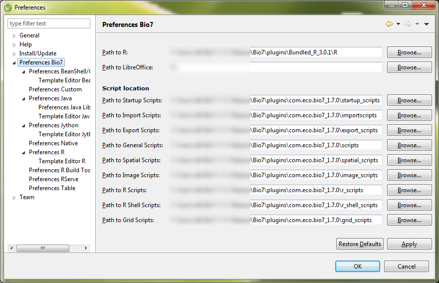
6.1.2 Script Paths
The following paths in the Preferences Bio7 are script path locations where scripts and macros (ImageJ macros) can be dropped which update the menu (except Startup Scripts!) of the Bio7 application at runtime (see 10.4↓). The import and export scripts will update the file menu. The other scripts and macros (General, R-Scripts, Spatial-Scripts, ImageJ-Macros, etc.) will update the scripts or special custom menus of Bio7.The locations of the scripts can be browsed easily with the browse action and files can be transferred simply by copy and paste from the Navigator. The files will be detected automatically and displayed in the appropriate menu for execution.
6.1.3 Bio7 Editor Preferences
The Preferences of the different language editors in Bio7 (R, BeanShell/Groovy, Java, Jython) offering methods to adjust the default colours and fonts and templates of the editors.
- Preferences Bio7 ▷ Preferences xxx-Editor for changing the default colours.
- Preferences Bio7 ▷ Preferences xxx-Editor ▷ Template Editor xxx to change the default templates.
It should be mentioned that some aspects of the language editors can be changed in the default text preferences of the platform (e.g. font attributes).
6.1.4 Preferences Rserve
As already described the preferences for the Rserve application (Preferences Bio7 ▷ Preferences Rserve or R ▷ Preferences) offers some options for code templates, editor colors and general adjustments (see ↓).
6.1.5 Default Platform Preferences
A detailed description of the preferences of the platform can be found on http://help.eclipse.org/.
7 Help
For a first help simply open the Bio7 browser Help ▷ Bio7 Internet By selecting the submenu Help ▷ Help Contents the Bio7 API can be opened in a HTML menu. The Welcome action opens a welcome page for the Bio7 application. The About Bio7 dialog opens an information about the current release of Bio7.
8 Update Manager
With the update manager Eclipse plugins can be easily installed or deleted. Update sites can be added as a installation source for existing external plugins. Installed third party plugins locations can be managed in the Available Software Sites preferences. Plugins can be deinstalled following the already installed link - it is even possible to return to a certain state of installation because the Eclipse Framework registers all configurations dates and changes. For more information about the update manager please consult the Eclipse documentation http://help.eclipse.org.
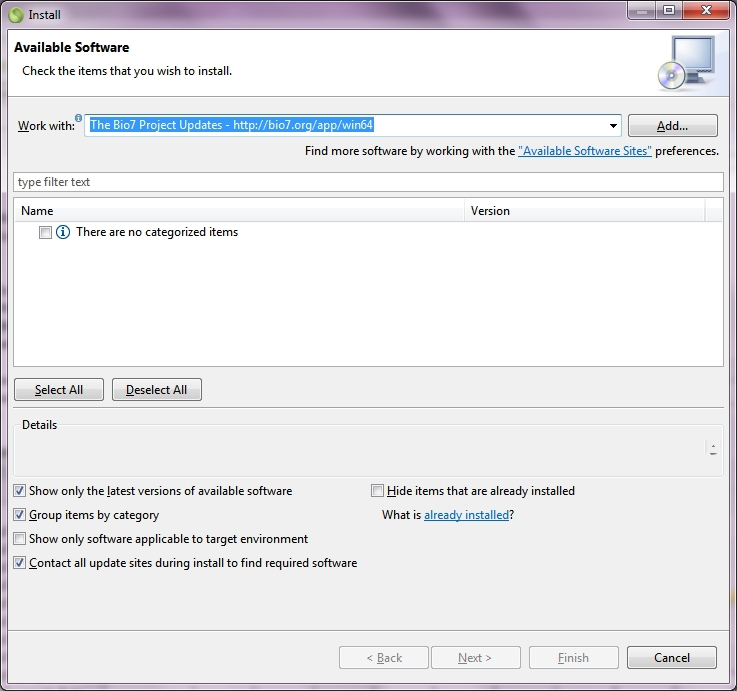
9 Additional Views and Interfaces
9.1 Additional Eclipse views in Bio7
By default some more views are available in Bio7:
- The Bookmarks view is a view which shows marked bookmarks in all language editors of Bio7 to easily find points in code which have to be edited.
- The Tasks view in the R-Editor serves as a marker for plots in the source code. For all other editors it can be used to leave some information about tasks that have to be done or as information in the Bio7 language editors (They can be marked with different priorities!).
- The Problems view to indicate compiler error and problems.
- The Cheat Sheets view can be used to load created Cheat Sheets from Eclipse.
- The Progress view shows information about running jobs in the application. Each time a job has started this progress view can be opened in the progress dialog of the status bar.
9.2 Java and Script Interaction with R
Additionally a nice feature in Bio7 is the direct interaction with the Rserve interpreter. Not only for evaluation, but also to obtain values from R to Java or BeanShell, Groovy and Jython is valuable for the creation and of models, etc. Not only a call to a R method is possible by means of compiled code but also calls from the BeanShell, Groovy and Jython interpreter can be made to transfer values e.g. to a BeanShell, Groovy, Jython workspace. R calculations can be interrupted (if supported by the package) with an opened system shell using the Strg+Break key combination on the shell (Windows), or with the pseudo terminal in in the Console view of Bio7 by typing: killall -INT Rserve (Linux, MacOSX). Because of the bidirectional transfer several things can be done, e.g.:
- Custom GUI’s can be created in Java or in the script interpreters and the values can be evaluated in R. After evaluation the results can be sent back to the interpreters workspace or to a method in Java.
- Build frontends for R methods with a scripted language (e.g. in JavaFX or SWT).
- Interaction between R and the API of ImageJ to automize image analysis tasks.
- Extend the script menus of Bio7 with R methods called by the script interpreters.
9.3 LibreOffice features of Bio7
If the free office software LibreOffice is installed, some methods for data acquisition and a small API for interaction with the LibreOffice spreadsheet are available in Bio7. To use the LibreOffice features it is necessary to establish a connection between LibreOffice and Bio7. This will be done automatically when selecting the action LibreOffice connection in the toolbar of Bio7. If a connection is established, several methods for the interaction with LibreOffice will be available in the LibreOffice menu.
- To receive or transfer values from or to the spreadsheet of LibreOffice it is necessary to open a spreadsheet. This can easily be done with the action LibreOffice ▷ Open Spreadsheet. After a spreadsheet has been opened (also possible by means of a small API) the spreadsheet can be filled with values by hand or with values from a file (in the opened spreadsheet menu of LibreOffice call the menu action: Insert ▷ Sheet from file).
- With the action Data to R LibreOffice spreadsheet values can be transferred to the active R workspace by means of the Rserve connection (the columns will be stored as lists and the selected values as a dataframe).
- With the action Data with head to R numeric values (type double) with a head can be transferred directly to R.
- With the action Send Bio7 counts counted values of the activated states in a simulation for all time steps are transferred to an opened spreadsheet which then can be stored to all kinds of data files.
- There is also a small API available for the transfer of data (get and set), inserting new sheets, getting values from sheets and the marking of the data in a spreadsheet (see Bio7 Snippets and Bio7 API docs).
10 What else ?
10.1 Native Preferences
In the native preferences some native connections to interpreters (R, Python) and OS shell preferences can be adjusted. The following preferences are available:
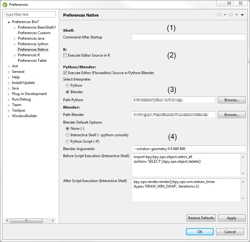
(1) With the Shell preferences the OS shell can be started within Bio7 with some arguments.
(2) In the R preference the R editor script can be executed with the native connection instead of the Rserve connection (deprecated - only useful if Rserve is started independent from the shell!).
(3) In the Python/Blender preference it can be adjusted to execute Python code of the editor with a native Python connection instead of the default Jython interpreter. The path to a Python interpreter has to be adjusted. In addition a Blender Python interpreter (which is embedded in an Blender installation) can be used to execute editor code. The different options are described in (4). Once again the path has to be adjusted.
(4) In the Blender Default Options some preferences can be selected and changed to start the Python interpreter and execute editor code in different ways.
- None will simply startup Blender without a Python script execution (arguments can be specified in the Blender Arguments).
- The option Interactive Shell if selected starts the Python connection as an interactiv shell (argument: --python-console). A special script customization is possible by defining code elements which will be executed before and after the editor code (the default code in the two textfields redraws the 3d GUI of Blender!)
- The option Python Script starts Blender and executes the editor script in Blender Python without an interactive shell.
- With the Blender Arguments additional arguments can be specified for the startup of Blender (e.g. with the option None some rendering tasks can be executed instead of executing a python script).
10.2 Drag, Drop, Compile and Start
Since Bio7 1.5 it is possible to store grid patterns in an *.xml file. If a Java editor is available the source code of an opened editor can be saved with the pattern. If source in a pattern file is available, too the source of the file will be loaded and compiled and the setup method (if available) will be executed. This can be used to execute a Java model with drag and drop. In addition this drag and drop action can also be used in conjunction with different java model types (3d models etc.). Please note that a package declaration in a Java file is not supported! Simply use the default /src project folder as created by the Bio7 project wizard when saving the file. Some examples can be found on GitHub: https://github.com/Bio7/Bio7
10.3 Drag and Drop Files
Several external file types can be dragged on the Bio7 interface. Here is an overview of the supported file types and the action involved:
| GUI Comp. | File Type | Action |
| Global (1) | *.exml | Loads a pattern, compiles Java code (if availabe) and executes the setup method of the compiled code. |
| Global (1) | *.RData | Starts Rserve (if not alive) and loads the *RData into the R workspace. |
| Navigator | *. | Copies all file types in a project of Bio7 (in the Bio7 workspace). |
| ImageJ-Canvas | *.png, *.jpg, etc. (2) | Opens images, stacks, etc. in the ImageJ view. |
| ImageJ-Canvas | *.jar | Installs and loads ImageJ plugins (default folder has to be selected). |
| ImageJ-Toolbar | *.png, *.jpg, etc. (2) | Opens images, stacks, etc. in the ImageJ view |
| Points | *.png, *.jpg, etc. (3) | Opens images in the Points panel and adjusts the “Area of Analysis”. |
Table 10.1 Drag And Drop actions in Bio7
(1) Except some Bio7 components with special drag and drop support and the editor area.
(2) All supported ImageJ file types and libs.
(3) Default Java supported image types.
10.4 Install Eclipse, R, ImageJ Plugins or Packages in Bio7
Bio7 can be extended in several different ways with Eclipse plugins, R packages, ImageJ plugins and custom scripts (scripts to extend a menu or executed at startup).
- To install (suitable) Eclipse plugins the Update-Manager can be used to install plugins from a remote website.
- R packages can be added in two different ways. One way is to use the package installer GUI of Bio7. Additionally the command line in R can be used to install packages.
- ImageJ plugins (*.class or *.jar files) have to be installed in the plugins folder of ImageJ which is is located in Bio7: Bio7/plugins/com.eco.bio7.image_x.xx.x/plugins. Note: In the ImageJ Eclipse plugin the typical ImageJ folder structure can be found!
- Groovy, BeanShell, Jython, JavaScript and R scripts, as well as ImageJ macros can be dropped to special folders to extend the default Bio7 menu (startup) functionality. The folders which are scanned by default are shown in the table below.
| Folder Location (see Preferences Bio7!) | Script Type | Menu | Bio7 Component |
| Bio7\plugins\com.eco.bio7_x.x.x\scripts | Java, BeanShell,Groovy, Jython, R, JavaScript, ImageJ Macro | Menu or submenus created from scripts and (nested) folders | Bio7 main menu |
| Bio7\plugins\com.eco.bio7_x.x.x\grid_scripts | Java, BeanShell,Groovy, Jython, R, JavaScript, ImageJ Macro | Menu or submenus created from scripts and (nested) folders | Table view menu |
| Bio7\plugins\com.eco.bio7_x.x.x\r_shell_scripts | Java, BeanShell,Groovy, Jython, R, JavaScript, ImageJ Macro | Menu or submenus created from scripts and (nested) folders | R-Shell context menu |
| Bio7\plugins\com.eco.bio7_x.x.x\startup_scripts | Groovy | Scripts executed at startup if option enabled | - |
Table 10.2 Scripts and their install locations for Bio7
10.5 Bio7 Themes
In Bio7 it is possible to select different themes. The default selected theme is the Bio7 theme. The theme can easily changed to a Bio7 dark theme by using the Window->Switch Theme action which also changes the editor font colors. In additon in the Bio7 preferences (Preferences->General->Appearence) other themes can be selected, too.
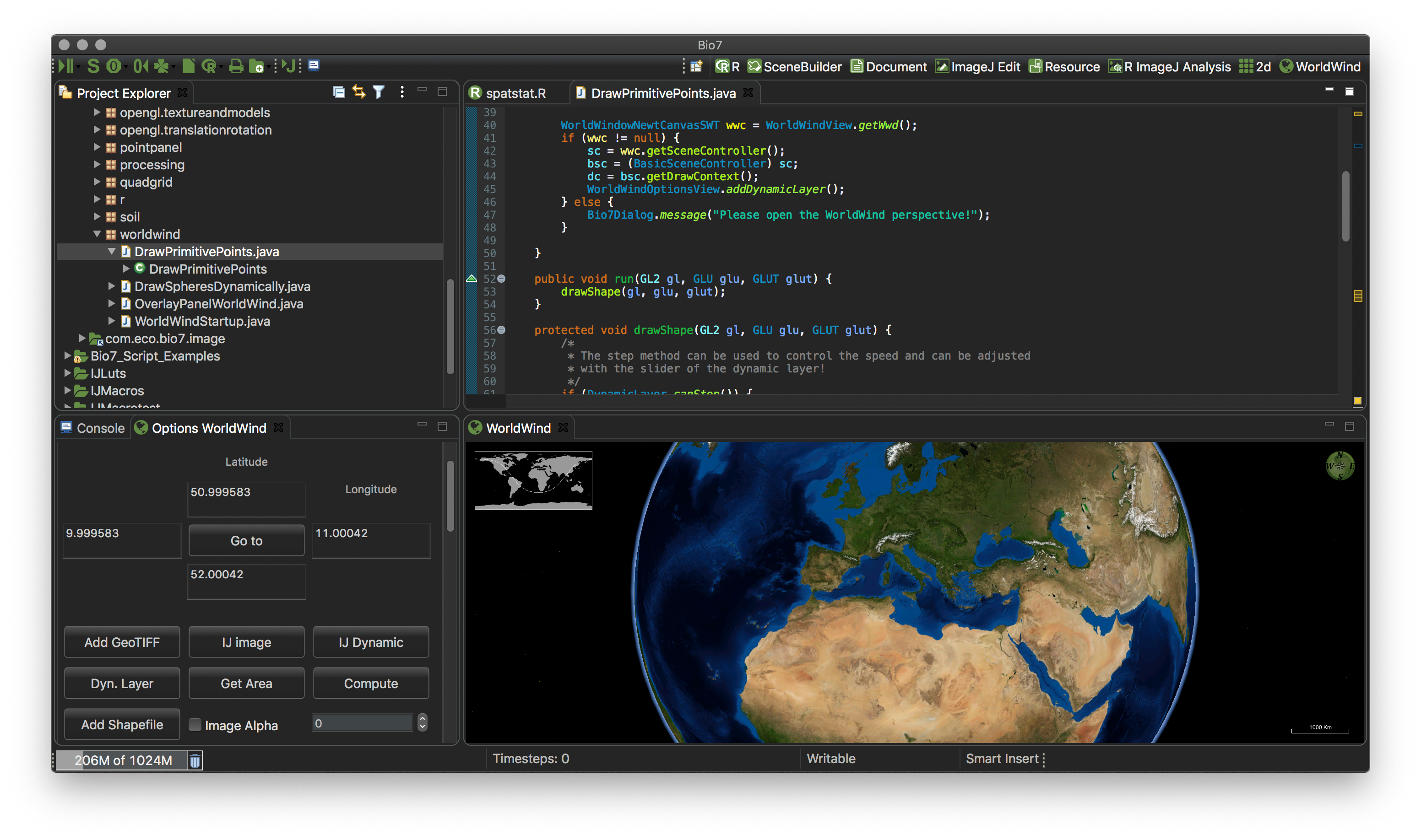
10.6 Install Git
One useful plugin for Bio7 is the Git plugin which can easily installed with the Update Manager of Bio7. Open the Update Manager and select the Update site for the plugin (see screenshot below). Then select the appropriate plugins. After installation a vast amounts of Git methods can be used easily with a Graphical User Interface. For a documentation please visit: http://www.eclipse.org/egit
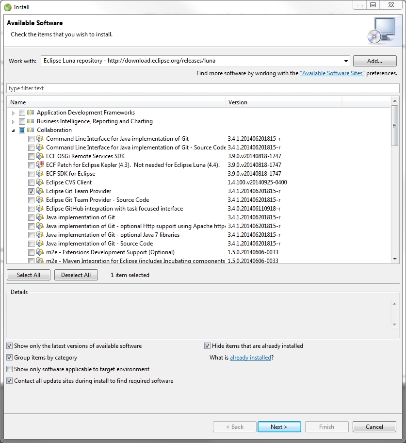
10.7 Bio7 Browser
Bio7 embeds the default Webbrowser engine in a view with custom links to useful developer resources for R, ImageJ, etc. The view can be opened in the Help menu (Help ▷ Bio7 Internet). In the Browser preferences of Bio7 another webbrowser type (JavaFX) can be selected for, e.g., the R help, rmarkdown, knitr documents (*.html, *.pdf).
10.8 Uninstall Eclipse Plugins
The about dialog embeds an action to uninstall installed Eclipse plugins or revert the installation of Bio7 to a specific date of installation. In this way a corrupted installation can be reverted to a previous state of installation.
10.9 Programming Examples for Bio7
The application Bio7 is distributed with a rich set of programming examples, which should facilitate the development of ecological models. The examples are so called Snippets (short programming examples) which are numbered and divided into two projects. One project (Bio7_Java_Examples) contains Java snippets for the different components of Bio7 which demonstrates how to use them and the flexibility of the platform in general. The other project Bio7_Script_Examples contains snippets as examples for the scripting languages. This Snippets also show that you can use the different embedded application and modules to understand and analyze complex systems or bundle them in ecological modeling for more complex purposes. The examples are available as projects. Please import them with File ▷ Import ▷ Existing Projects into Workspace into your Bio7 workspace. The Snippets can also be browsed and downloaded on github: https://github.com/Bio7.
11 Literature and Links
11.1 Scientific Libraries Available in Bio7
- JScience http://jscience.org/
- Colt http://dsd.lbl.gov/~hoschek/colt/
- Math http://jakarta.apache.org/commons/math/
- Weka http://www.cs.waikato.ac.nz/ml/weka/
- JTS http://www.vividsolutions.com/jts/JTSHome.htm
- Joone http://sourceforge.net/projects/joone/ JDMP http://www.jdmp.org/
11.2 Documentation and Programming Links:
- BeanShell http://www.beanshell.org/
- R http://www.r-project.org/
- Rserve http://www.rforge.net/Rserve/
- ImageJ http://rsb.info.nih.gov/ij/
- JavaCompiler http://www.janino.net/
- Groovy http://groovdehaus.org/
- Forums http://www.nabble.com (search for the different applications BeanShell, R, ImageJ, Janino)
12 Addendum
With an ID perspectives and views can be opened or closed programmatically. Below the ID’s of the perspectives and views are listed.
| View | Id |
| Space | com.eco.bio7.spatial |
| Options Space | com.eco.bio7.discrete3d.Options3d |
| 3Dgrid | com.eco.bio7.3d |
| Piechart | com.eco.bio7.piechart |
| Linechart | com.eco.bio7.linechart |
| Quadgrid | com.eco.bio7.quadgrid |
| Spreadsheet | com.eco.bio7.spreadsheet |
| State | com.eco.bio7.states |
| Hexgrid | com.eco.bio7.hexgrid |
| Custom Chart | com.eco.bio7.custom_chart |
| Points | com.eco.bio7.points |
| Image-Methods | com.eco.bio7.image_methods |
| Bsh-Console | com.eco.bio7.bsh |
| Control | com.eco.bio7.control |
| Browser | com.eco.bio7.browser.Browser |
| Browser Editor | com.eco.bio7.browser.BrowserEditorView |
| WorldWind | com.eco.bio7.worldwind.WorldWindView |
| Options WorldWind | com.eco.bio7.worldwind.WorldWindOptionsView |
| Custom Controlls | com.eco.bio7.custom_controls |
| Custom 3d | com.eco.bio7.custom_3d |
| Navigator | org.eclipse.ui.views.ResourceNavigator |
| Progress | org.eclipse.ui.views.ProgressView |
| Bookmark | org.eclipse.ui.views.BookmarkView |
| Tasks | org.eclipse.ui.views.TaskList |
| Problems | org.eclipse.ui.views.ProblemView |
| Console | org.eclipse.ui.console.ConsoleView |
| Properties | org.eclipse.ui.views.PropertySheet |
| Outline | org.eclipse.ui.views.ContentOutline |
| R-Shell | com.eco.bio7.RShell |
| Table | com.eco.bio7.rbridge.RTable |
| ImageJ-Canvas | com.eco.bio7.imagej |
| Geometry Selections | com.eco.bio7.image.TransferGeometryView |
| Debug (x) | com.eco.bio7.rbridge.debug.DebugVariablesView |
| Debug Text | com.eco.bio7.rbridge.debug.DebugTextView |
| Custom Controls | com.eco.bio7.custom_controls |
| Hierachy | com.eco.bio7.scenebuilder.hierachy |
| Library | com.eco.bio7.scenebuilder.library |
| Inspector | com.eco.bio7.scenebuilder.inspector |
| Css | com.eco.bio7.scenebuilder.css |
Table 12.1 View ID to call programmatically
- To use programmatically: Work.openView("Id");
- Example: Work.openView("com.eco.bio7.quadgrid");
| Perspective | ID |
| 2D | com.eco.bio7.perspective_2d |
| 3D | com.eco.bio7.perspective_3d |
| R | com.eco.bio7.rbridge.RPerspective |
| Image | com.eco.bio7.perspective_image |
| Web | com.eco.bio7.browser.HtmlEditorPerspective |
| Resource | org.eclipse.ui.resourcePerspective |
| WorldWind | com.eco.bio7.WorldWind.3dglobe |
| Custom | com.eco.bio7.CustomPerspective |
| SceneBuilder | com.eco.bio7.browser.SceneBuilderPerspective |
Table 12.2 Perspective ID to call programmatically
- To use programmatically: Work.openPerspective("Id");
- Example: Work.openPerspective("com.eco.bio7.perspective_2d");
- A saved custom perspective is available by it’s name !
- Example: Work.openPerspective("Custom"); //if saved as “Custom”
- Bio7 API : A small API is integrated in Bio7. The API is available within the help of Bio7.
13 Definition of Expressions
- Area of Analysis: A name for the area in the Points panel which is marked by a green rectangle for spatial point patterns.
- Programmatically: Using programming to accomplish a task.
- Namespace (BeanShell) : A namespace in which methods, variables, and imports (class names) live.
- Workspace (R): A saveable environment in which methods, variables and objects exists.
- Workspace (Bio7): The location where the projects and files are stored.
- Calculation thread: A time dependent execution of a compiled method (ecomain) in Bio7 started, e.g. with the Play/Pause button.
- Discretize: In Bio7 the process of transferring continuous data to discrete data.
- IDE (Integrated Development Environment): a type of software that assists in developing software.
- Snippets: In Bio7 a small piece of programming source code to demonstrate some of the Bio7 features.
Bibliography
[1] . Spatiotemporal models of population and community dynamics. Chapman & Hall, 1998.
[2] . The geometry of ecological interactions: simplifying spatial complexity. Cambridge University Press, 2000.
[3] . A Primer of Ecology, Fourth Edition. Sinauer Associates, Inc., may 2008.
[4] . Modeling Biological Systems:: Principles and Applications. Springer, may 2005.
[5] . Handbook of ecological modelling and informatics. WIT Press, feb 2009.
[6] . The Science of Fractal Images. In (Peitgen, Heinz-Otto and Saupe, Dietmar, ed.). Springer-Verlag New York, Inc., 1988. URL http://dl.acm.org/citation.cfm?id=61153.61156.
[7] . Environmental Modelling: Finding Simplicity in Complexity. Wiley, jan 2004.
List of Figures